Artificial Neural Networks#
%matplotlib inline
import matplotlib.pyplot as plt
import seaborn as sns; sns.set_theme()
import numpy as np
import pandas as pd
import torch.nn
import functools
import copy
import warnings
warnings.filterwarnings('ignore')
# Use CPU rather than GPU for keras neural networks
import os
os.environ["CUDA_DEVICE_ORDER"] = "PCI_BUS_ID"
os.environ["CUDA_VISIBLE_DEVICES"] = ""
from tensorflow import keras
from tqdm.keras import TqdmCallback
2026-02-16 21:02:14.115156: I tensorflow/core/util/port.cc:153] oneDNN custom operations are on. You may see slightly different numerical results due to floating-point round-off errors from different computation orders. To turn them off, set the environment variable `TF_ENABLE_ONEDNN_OPTS=0`.
2026-02-16 21:02:14.143074: I tensorflow/core/platform/cpu_feature_guard.cc:210] This TensorFlow binary is optimized to use available CPU instructions in performance-critical operations.
To enable the following instructions: AVX2 AVX512F AVX512_VNNI AVX512_BF16 AVX_VNNI FMA, in other operations, rebuild TensorFlow with the appropriate compiler flags.
2026-02-16 21:02:14.768067: I tensorflow/core/util/port.cc:153] oneDNN custom operations are on. You may see slightly different numerical results due to floating-point round-off errors from different computation orders. To turn them off, set the environment variable `TF_ENABLE_ONEDNN_OPTS=0`.
Below we inlucde a set of helper functions to visualize the calculations for illustration purposes:
def nn_map2d(fx, params=None, x_range=3, ax=None, vlim=None, label=None):
    """
    """
    ax = ax or plt.gca()
    if vlim is None:
        vlim = np.max(np.abs(fx))
    ax.imshow(fx, interpolation='none', origin='lower', cmap='coolwarm',
              aspect='equal', extent=[-x_range, +x_range, -x_range, +x_range],
              vmin=-vlim, vmax=+vlim)
    if params:
        w, b = params
        w = np.asarray(w)
        x0 = -b * w / np.dot(w, w)
        ax.annotate('', xy=x0 + w, xytext=x0,
                    arrowprops=dict(arrowstyle='->', lw=3, color='k'))
    if label:
        ax.text(0.5, 0.9, label, horizontalalignment='center',
                color='k', fontsize=16, transform=ax.transAxes)
    ax.grid(False)
    ax.axis('off')


def nn_unit_draw2d(w, b, phi, x_range=3, nx=250, ax=None, vlim=None, label=None):
    """Draw a single network unit or layer with 2D input.

    Parameters
    ----------
    w : array
        1D array of weight values to use.
    b : float or array
        scalar (unit) or 1D array (layer) of bias values to use.
    phi : callable
        Activation function to use.
    """
    x_i = np.linspace(-x_range, +x_range, nx)
    X = np.stack(np.meshgrid(x_i, x_i), axis=2).reshape(nx ** 2, 2)
    W = np.asarray(w).reshape(2, 1)
    fx = phi(np.dot(X, W) + b).reshape(nx, nx)
    nn_map2d(fx, (w, b), x_range, ax, vlim, label)


def nn_graph_draw2d(*layers, x_range=3, label=None, n_grid=250, n_bins=25):
    """Draw the response of a neural network with 2D input.

    Parameters
    ----------
    *layers : tuple
        Each layer is specified as a tuple (W, b, phi).
    """
    x_i = np.linspace(-x_range, +x_range, n_grid)
    layer_in = np.stack(np.meshgrid(x_i, x_i), axis=0).reshape(2, -1)
    layer_out = [ ]
    layer_s = [ ]
    depth = len(layers)
    n_max, vlim = 0, 0.
    for i, (W, b, phi) in enumerate(layers):
        WT = np.asarray(W).T
        b = np.asarray(b)
        n_out, n_in = WT.shape
        n_max = max(n_max, n_out)
        if layer_in.shape != (n_in, n_grid ** 2):
            raise ValueError(
                'LYR{}: number of rows in W ({}) does not match layer input size ({}).'
                .format(i + 1, n_in, layer_in.shape))
        if b.shape != (n_out,):
            raise ValueError(
                'LYR{}: number of columns in W ({}) does not match size of b ({}).'
                .format(i + 1, n_out, b.shape))
        s = np.dot(WT, layer_in) + b.reshape(-1, 1)
        layer_s.append(s)
        layer_out.append(phi(s))
        layer_in = layer_out[-1]
        vlim = max(vlim, np.max(layer_in))
    _, ax = plt.subplots(n_max, depth, figsize=(3 * depth, 3 * n_max),
                         sharex=True, sharey=True, squeeze=False)
    for i, (W, b, phi) in enumerate(layers):
        W = np.asarray(W)
        for j in range(n_max):
            if j >= len(layer_out[i]):
                ax[j, i].axis('off')
                continue
            label = 'LYR{}-NODE{}'.format(i + 1, j + 1)
            params = (W[:,j], b[j]) if i == 0 else None
            fx = layer_out[i][j]
            nn_map2d(fx.reshape(n_grid, n_grid), params=params,
                      ax=ax[j, i], vlim=vlim, x_range=x_range, label=label)
            if i > 0 and n_bins:
                s = layer_s[i][j]
                s_min, s_max = np.min(s), np.max(s)
                t = 2 * x_range * (s - s_min) / (s_max - s_min) - x_range
                rhs = ax[j, i].twinx()
                hist, bins, _ = rhs.hist(
                    t, bins=n_bins, range=(-x_range, x_range),
                    histtype='stepfilled', color='w', lw=1, alpha=0.25)
                s_grid = np.linspace(s_min, s_max, 101)
                t_grid = np.linspace(-x_range, +x_range, 101)
                phi_grid = phi(s_grid)
                phi_min, phi_max = np.min(phi_grid), np.max(phi_grid)
                z_grid = (
                    (phi_grid - phi_min) / (phi_max - phi_min) * np.max(hist))
                rhs.plot(t_grid, z_grid, 'k--', lw=1, alpha=0.5)
                rhs.axvline(-x_range * (s_max + s_min) / (s_max - s_min),
                            c='w', lw=1, alpha=0.5)
                rhs.set_xlim(-x_range, +x_range)
                rhs.axis('off')
    plt.subplots_adjust(wspace=0.015, hspace=0.010,
                        left=0, right=1, bottom=0, top=1)

def sizes_as_string(tensors):
    if isinstance(tensors, torch.Tensor):
        return str(tuple(tensors.size()))
    else:
        return ', '.join([sizes_as_string(T) for T in tensors])

def trace_forward(module, input, output, name='', verbose=False):
    """Implement the module forward hook API.

    Parameters
    ----------
    input : tuple or tensor
        Input tensor(s) to this module. We save a detached
        copy to this module's `input` attribute.
    output : tuple or tensor
        Output tensor(s) to this module. We save a detached
        copy to this module's `output` attribute.
    """
    if isinstance(input, tuple):
        module.input = [I.detach() for I in input]
        if len(module.input) == 1:
            module.input = module.input[0]
    else:
        module.input = input.detach()
    if isinstance(output, tuple):
        module.output = tuple([O.detach() for O in output])
        if len(module.output) == 1:
            module.output = module.output[0]
    else:
        module.output = output.detach()
    if verbose:
        print(f'{name}: IN {sizes_as_string(module.input)} OUT {sizes_as_string(module.output)}')

def trace_backward(module, grad_in, grad_out, name='', verbose=False):
    """Implement the module backward hook API.

    Parameters
    ----------
    grad_in : tuple or tensor
        Gradient tensor(s) for each input to this module.
        These are the *outputs* from backwards propagation and we
        ignore them.
    grad_out : tuple or tensor
        Gradient tensor(s) for each output to this module.
        Theser are the *inputs* to backwards propagation and
        we save detached views to the module's `grad` attribute.
        If grad_out is a tuple with only one entry, which is usually
        the case, save the tensor directly.
    """
    if isinstance(grad_out, tuple):
        module.grad = tuple([O.detach() for O in grad_out])
        if len(module.grad) == 1:
            module.grad = module.grad[0]
    else:
        module.grad = grad_out.detach()
    if verbose:
        print(f'{name}: GRAD {sizes_as_string(module.grad)}')

def trace(module, active=True, verbose=False):
    if hasattr(module, '_trace_hooks'):
        # Remove all previous tracing hooks.
        for hook in module._trace_hooks:
            hook.remove()
    if not active:
        return
    module._trace_hooks = []
    for name, submodule in module.named_modules():
        if submodule is module:
            continue
        module._trace_hooks.append(submodule.register_forward_hook(
            functools.partial(trace_forward, name=name, verbose=verbose)))
        module._trace_hooks.append(submodule.register_full_backward_hook(
            functools.partial(trace_backward, name=name, verbose=verbose)))


def get_lr(self, name='lr'):
    lr_grps = [grp for grp in self.param_groups if name in grp]
    if not lr_grps:
        raise ValueError(f'Optimizer has no parameter called "{name}".')
    if len(lr_grps) > 1:
        raise ValueError(f'Optimizer has multiple parameters called "{name}".')
    return lr_grps[0][name]

def set_lr(self, value, name='lr'):
    lr_grps = [grp for grp in self.param_groups if name in grp]
    if not lr_grps:
        raise ValueError(f'Optimizer has no parameter called "{name}".')
    if len(lr_grps) > 1:
        raise ValueError(f'Optimizer has multiple parameters called "{name}".')
    lr_grps[0][name] = value

# Add get_lr, set_lr methods to all Optimizer subclasses.
torch.optim.Optimizer.get_lr = get_lr
torch.optim.Optimizer.set_lr = set_lr

def lr_scan(loader, model, loss_fn, optimizer, lr_start=1e-6, lr_stop=1., lr_steps=100):
    """Implement the learning-rate scan described in Smith 2015.
    """
    import matplotlib.pyplot as plt
    # Save the model and optimizer states before scanning.
    model_save = copy.deepcopy(model.state_dict())
    optim_save = copy.deepcopy(optimizer.state_dict())
    # Schedule learning rate to increase in logarithmic steps.
    lr_schedule = np.logspace(np.log10(lr_start), np.log10(lr_stop), lr_steps)
    model.train()
    losses = []
    scanning = True
    while scanning:
        for x_in, y_tgt in loader:
            optimizer.set_lr(lr_schedule[len(losses)])
            y_pred = model(x_in)
            loss = loss_fn(y_pred, y_tgt)
            losses.append(loss.data)
            if len(losses) == lr_steps or losses[-1] > 10 * losses[0]:
                scanning = False
                break
            optimizer.zero_grad()
            loss.backward()
            optimizer.step()
    # Restore the model and optimizer state.
    model.load_state_dict(model_save)
    optimizer.load_state_dict(optim_save)
    # Plot the scan results.
    plt.plot(lr_schedule[:len(losses)], losses, '.')
    plt.ylim(0.5 * np.min(losses), 10 * losses[0])
    plt.yscale('log')
    plt.xscale('log')
    plt.xlabel('Learning rate')
    plt.ylabel('Loss')
    # Return an optimizer with set_lr/get_lr methods, and lr set to half of the best value found.
    idx = np.argmin(losses)
    lr_set = 0.5 * lr_schedule[idx]
    print(f'Recommended lr={lr_set:.3g}.')
    optimizer.set_lr(lr_set)
Overview#
From a user’s perspective, a neural network (NN) is a class of models
that are:
Generic: they are not tailored to any particular application.
Flexible: they can accurately represent a wide range of non-linear \(X_\text{in}\rightarrow X_\text{out}\) mappings with a suitable choice of parameters \(\Theta\).
Trainable: a robust optimization algorithm (backpropagation) can learn parameters \(\Theta\) given enough training data \(D = (X_\text{in},Y_\text{tgt})\).
Modular: it is straightforward to scale the model complexity (and number of parameters) to match the available training data.
Efficient: most of the internal computations are linear and amenable to parallel computation and hardware acceleration.
The “neural” aspect of a NN is tenuous. Their design mimics some aspects of biological neurons, but also differs in fundamental ways.
In this notebook, we will explore NNs from several different perspectives:
Mathematical: What equations describe a network?
Visual: What does the network graph look like? How is the input space mapped through the network?
Data Flow: What are the tensors that parameterize and flow (forwards and backwards) through a network?
Statistical: What are typical distributions of tensor values?
Mathematical Perspective#
Building Block#
The internal structure of a NN is naturally described by a computation graph that connects simple building blocks. The basic building-block unit is a function of \(D\) input features \(x_i\),
with \(D+1\) parameters consisting of \(D\) weights \(w_i\) and a single bias \(b\). The corresponding graph (with \(D=8\)) is:
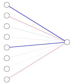
where the left nodes correspond to the elements of the input \(\mathbf{x}\), the edges correspond to the elements of \(\mathbf{w}\) (thickness ~ strength, red/blue are pos/neg values), and the right node is the output value \(f(\mathbf{x})\). The recipe for obtaining the output value is then:
propagate each input value \(x_i\) with a strength \(w_i\),
sum the values \(x_i w_i\),
add a bias value \(b\)
apply the activation \(\phi\).
Note that this building block is mostly linear, except for the activation function \(\phi(s)\). This is an application of the kernel trick that we met earlier, and allows us to implicitly work in a higher dimensional space where non-linear structure in data is easier to model.
The building-block equation is straightfoward to implement as code:
def nn_unit(x, w, b, phi):
    return phi(np.dot(x, w) + b)
For example, with a 3D input \(\mathbf{x}\), the weight vector \(\mathbf{w}\) should also be 3D:
nn_unit(x=[0, 1, -1], w=[1, 2, 3], b=-1, phi=np.tanh)
np.float64(-0.9640275800758169)
Activation Functions#
The activation function \(\phi\) argument \(s\) is always a scalar and, by convention, activation functions are always defined in a standard form, without any parameters (since \(\mathbf{w}\) and \(b\) already provide enough learning flexibility).
Some popular activations are defined below (using lambda functions). For the full list supported in PyTorch see here.
relu     = lambda s: np.maximum(0, s)
elu      = lambda s: np.maximum(0, s) + np.minimum(0, np.expm1(s)) # expm1(s) = exp(s) - 1
softplus = lambda s: np.log(1 + np.exp(s))
sigmoid  = lambda s: 1 / (1 + np.exp(-s)) # also known as the "logistic function"
tanh     = lambda s: np.tanh(s)
softsign = lambda s: s / (np.abs(s) + 1)
These activations divide naturally into two categories depending on their asymptotic behavior as \(s\rightarrow +\infty\):
def plot_activations(ax, names, s_range=5, y_range=2):
    s = np.linspace(-s_range, +s_range, 101)
    for name in names.split(','):
        phi = eval(name)
        ax.plot(s, phi(s), lw=4, alpha=0.5, label=name)
    ax.legend(fontsize='x-large')
    ax.set_xlabel('Activation input $s$')
    ax.set_ylabel('Activation output $\phi(s)$')
    ax.set_xlim(-s_range, +s_range)
    ax.set_ylim(-y_range, +y_range)
    ax.axhline(-1, c='gray', ls=':')
    ax.axhline(+1, c='gray', ls=':')

_, ax = plt.subplots(1, 2, figsize=(12, 5))
plot_activations(ax[0], 'relu,elu,softplus')
plot_activations(ax[1], 'sigmoid,tanh,softsign')
plt.tight_layout()
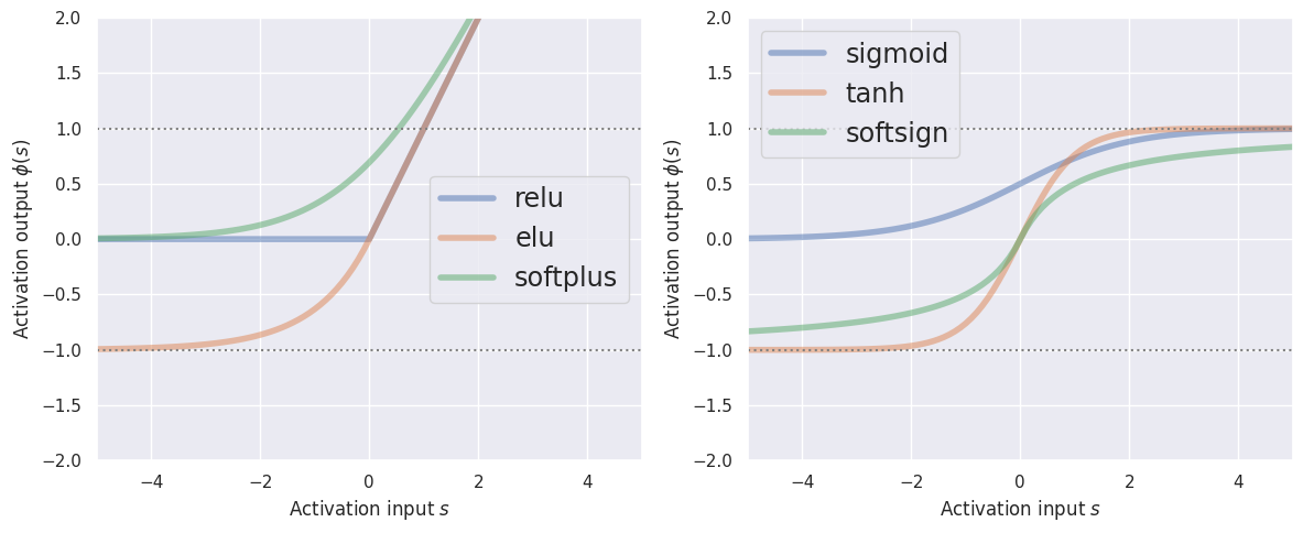
Note that all activations saturate (at -1 or 0) for \(s\rightarrow -\infty\), but differ in their behavior when \(s\rightarrow +\infty\) (linear vs saturate at +1).
DISCUSS:
Which activation would you expect to be the fastest to compute?
Which activations are better suited for a binary classification problem?
The relu activation is the fastest to compute since it does not involve any transcendental function calls (exp, log, …).
The activations that are bounded on both sides only have a narrow range near \(s=0\) where they distinguish between different input values, and otherwise are essentially saturated at one of two values. This is desirable for classification, where the aim is to place \(s=0\) close to the “decision boundary” (by learning a suitable bias).
Network Layer#
What happens if we replace the vectors \(\mathbf{x}\) and \(\mathbf{w}\) above with matrices?
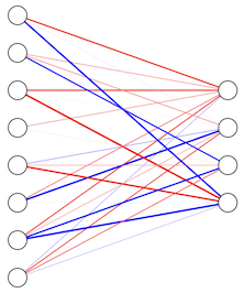
If \(X\) has shape \((N, D)\) and holds \(N\) samples of \(D\) features, then \(W\) must have shape \((D, M)\) so \(F(X)\) converts the \(D\) input features into \(M\) output features for each sample. We say that \(F\) represents a linear network layer with \(D\) input nodes and \(M\) output nodes. Note that the bias is now a vector of \(M\) bias values, one for each output value.
We cannot really add a vector \(\mathbf{b}\) to the matrix \(X W\) but we are using the “broadcasting” convention that this means add the same vector to each row (sample) of \(X W\). We also cannot apply \(\phi(s)\) to a matrix, but we are using the “elementwise” convention that this means apply \(\phi\) separately to each element of the matrix.
To connect this matrix version with our earlier vector version, notice that \(F(X)\) transforms a single input sample \(\mathbf{x}_i\) (row of \(X\)) into \(M\) different outputs, \(f_m(\mathbf{x}_i)\) each with their own weight vector and bias value:
where \(\mathbf{w}_m\) is the \(m\)-th column of \(W\) and \(b_m\) is the \(m\)-th element of \(\mathbf{b}\).
The corresponding graph (with \(D=8\) and \(M=4\)) is:
The nn_unit function we defined above already implements a layer if we pass it matrices \(X\) and \(W\) and a vector \(\mathbf{b}\). For example:
nn_unit(x=[[1., 0.5], [-1, 1]], w=[[1, -1, 1], [2, 0, 1]], b=[-1, 1, 0], phi=sigmoid)
array([[0.73105858, 0.5       , 0.81757448],
       [0.5       , 0.88079708, 0.5       ]])
A layer with \(n_{in}\) inputs and \(n_{out}\) outputs has a total of \((n_{in} + 1) ~n_{out}\) parameters. These can add up quickly when building useful networks!
Network Graph#
Finally, we can build a simple fully connected graph by stacking layers horizontally, which corresponds to nested calls of each layer’s function. For example, with 3 layers computed by \(F\), \(G\), \(H\) stacked (left to right), the overall graph computation is:
with a corresponding graph:
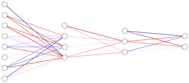
Nodes between the input (leftmost) and output (rightmost) nodes are known as hidden nodes.
The corresponding code for arbitrary layers is:
def nn_graph(X, *layers):
    for W, b, phi in layers:
        X = nn_unit(X, W, b, phi)
    return X
For example, here is a three-layer network with the same architecture as the graph above. Note how the output dimension of one layer must match the input dimension of the next layer.
nn_graph([1, 2, 3, 4, 5, 6, 7, 8],
    ([
        [11, 12, 13, 14],
        [21, 22, 23, 24],
        [31, 32, 33, 34],
        [41, 42, 43, 44],
        [51, 52, 53, 54],
        [61, 62, 63, 64],
        [71, 72, 73, 74],
        [81, 82, 83, 84],
    ], [1, 2, 3, 4], tanh),    # LYR1: n_in=8, n_out=4
    ([
        [11, 12, 13],
        [21, 22, 23],
        [31, 32, 33],
        [41, 42, 43],
    ], [1, 2, 3], relu),       # LYR2: n_in=4, n_out=3
    ([
        [11, 12],
        [21, 22],
        [31, 32],
    ], [1, 2], sigmoid)        # LYR3: n_in=3, n_out=2
)
array([1., 1.])
The weight and bias values are chosen to make the tensors easier to read, but would not make sense for a real network. As a result, the final output of [1., 1.] is not surprising given how the sigmoid activation saturates for input outside a narrow range.
Visual Perspective#
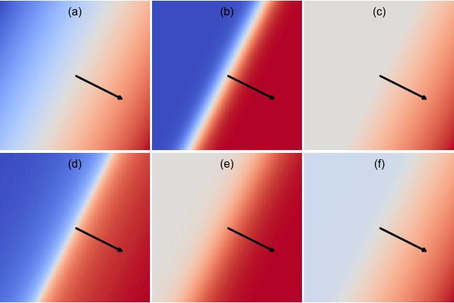
EXERCISE: Identify which activation function was used to make each plot above, which shows the building block
for a 2D \(\mathbf{x}\) with the same \(\mathbf{w}\) and \(b\) used in each plot. Red and blue indicate positive and negative values, respectively, with zero displayed as white. For calibration, (a) shows a “linear” activation which passes its input straight through.
(a) linear
(b) tanh
(c) relu
(d) softsign
(e) sigmoid
(f) elu
To distinguish between (b) and (d), note that both go asymptotically to constant negative and positive values (so sigmoid is ruled out), but the white transition region is narrower for (d).
To distinguish between (c) and (f), note that (c) goes asymptotically to zero (white) in the top-left corner, while (e) goes asymptotically to a constant negative value (blue).
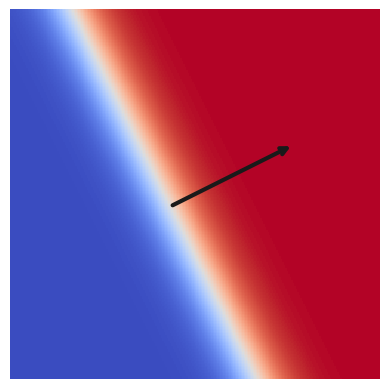
EXERCISE: Experiment with the following function to determine how the displayed arrow relates to the three model parameters \(w_0, w_1, b\):
nn_unit_draw2d(w=[0, 2], b=-1, phi=tanh)
The arrow has the direction and magnitude of the 2D vector \(\mathbf{w}\), with its origin at \(\mathbf{x} = -b \mathbf{w}\, / \, |\mathbf{w}|^2\) where \(s = 0\). The line \(s=0\) is perpendicular to the arrow.
nn_unit_draw2d(w=[2, 1], b=+1, phi=tanh)
Study the plots below which show the hidden (left) and output (right) node values for a network with 2 + 2 + 1 nodes. Each graph shows the node value as a function of the 2D input value.
Note how the hidden nodes divide the input space into two halves, with a dividing line determined by their \(\mathbf{w}\) and \(b\) values. The output layer then mixes these halves and can therefore “select” any of the four quadrants with an appropriate choice of its \(\mathbf{w}\) and \(b\).
nn_graph_draw2d(
    ([[2, 0],[-1, -2]], [0, 0], tanh), # LYR1
    ([[1], [-1]], [-1], tanh)          # LYR2
)
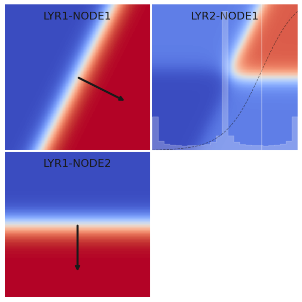
The histogram on the second layer plot shows the distribution of
feeding its activation function (shown as the dashed curve). Note how the central histogram peak is higher because both the lower-right and upper-left quadrants of \((x_1, x_2)\) have \(Y W \simeq 0\). The vertical white line shows how our choice of bias \(b = -0.5\) places these quadrants in the “rejected” (blue) category with \(s < 0\).
Generalizing this example, a layer with \(n\) inputs can “select” a different \(n\)-sided (soft-edged) polygon with each of its outputs. To see this in action, try this demo.
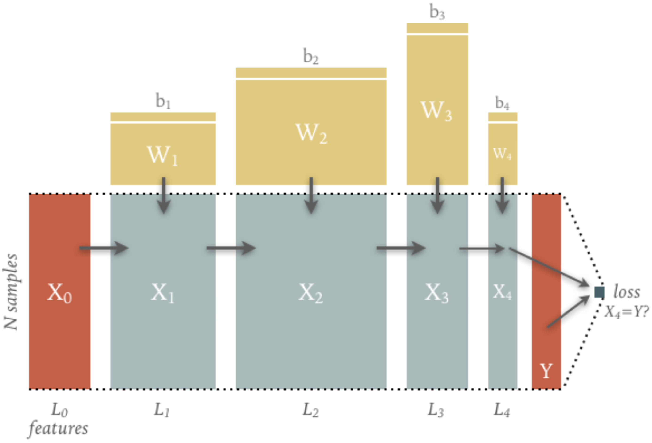
Data Flow Perspective#
The diagram below show the tensors flowing forward (left to right) in a typical fully connected graph. The main flow consists of \(N\) input samples flowing from \(X_0\) to \(X_4\) with a number of features that varies between layers.
The computation of each layer’s output is parameterized by the weight and bias tensors shown: note how their shapes are determined by the number of input and output features for each layer. The parameter tensors are usually randomly initialized (more on this soon) so only the input \(X_0\) and target \(Y\) are needed to drive the calculation (and so must be copied to GPU memory when using hardware acceleration).
The final output \(X_4\) is compared with the target values \(Y\) to calculate a “loss” \(\ell(X_4, Y)\) that decreases as \(X_4\) becomes more similar to \(Y\) (more on this soon).
The diagram below shows the gradient (partial derivative) tensors flowing backwards (“backpropagation”) through the same graph using the chain rule:
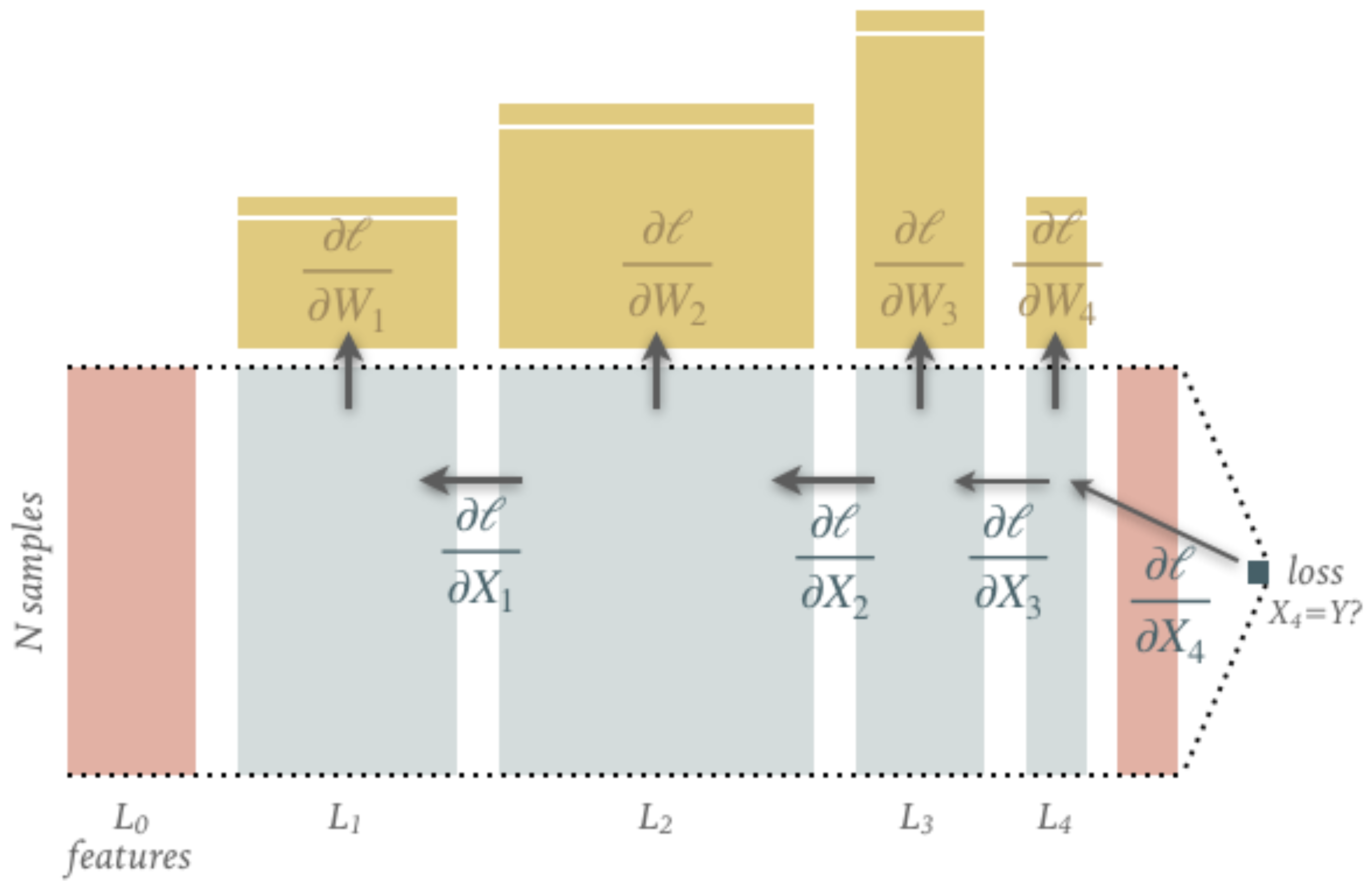
Note that these gradient tensors are just numbers, not functions. All of these tensors occupy the (limited) GPU memory when using hardware acceleration but, in most applications, only the final output and the parameter gradients are stored (with 32-bit floating point precision).
When working with large datasets, the \(N\) input samples are usually broken up into fixed-size randomly subsampled “minibatches”. Optimiztion with the resulting parameter gradients leads to the “stochastic gradient descent” (SGD) algorithm.
Feedforward Neural Network: Keras and Tensorflow#
A feedforward neural network is a function that was designed to mimic biological neural networks. It can be written as simply
This may look confusing at first glance, but basically it is just a function that takes in a vector (or value) \(\textbf{x}\) and outputs a value \(y\).
This function is a nested function (in that it repeatedly applies the function \(f\)) and can be written more legibly as:
Note that at the \(i^\text{th}\) level, \(y_{i-1}\) is the input to the function.
Structure#
You may be wondering how this is similar to biological neural networks. This is clearer if we write the above in a diagram form:

For some terminology,
\(f\) is an “activation” function (something like \(\tanh\))
\(W_i\) is called a “weight” matrix
\(b_i\) is called a “bias” vector
Because \(W_i\) are matrices, they can change the dimension at each level. For example, if our input \(\textbf{x}\) was a vector of 3 items, and the matrix \(W_1\) was a \(5 \times 3\) matrix, then \(W_1\textbf{x}\) would be a size 5 vector. With this in mind, the above diagram is more commonly drawn as:

This diagram shows how the function we wrote above is actually a network. Each line on the diagram represents an operation like \(W_{i,jk}y_{i,k} + b_j\) where \(W_{i,jk}\) is the \(j,k\) entry in the \(W_i\) matrix. Each circle is the application of the activation function \(f\) (which could actually be different at each layer) and are usually called “nodes.” The network is called “feedforward” because data only flows from left to right (there are no loops).
Let’s create a simple network with the following properties in the keras Python framework:
\(\textbf{x}\) is a vector of length 2
\(W_1,W_2\) are sizes \(3\times 2\) and \(1 \times 3\) respectively
\(b_1, b_2\) are vectors of size \(3\) and \(1\) respectively
\(f\) is a \(\tanh\) function
# Set the random seed to make sure we get reproducible results (we get the same every time we run)
keras.utils.set_random_seed(0)

# Make input layer of appropriate size (1 sample of size 2)
x   = keras.layers.Input(shape=(2,),name="Input")

# Pass input x into first layer of size 3 x 2
y_1 = keras.layers.Dense(3,activation="tanh")(x)

# Pass middle or "hidden" layer into output
y   = keras.layers.Dense(1,activation="tanh")(y_1)

model = keras.Model(inputs=x,outputs=y)
2026-02-16 21:02:15.207089: E external/local_xla/xla/stream_executor/cuda/cuda_platform.cc:51] failed call to cuInit: INTERNAL: CUDA error: Failed call to cuInit: CUDA_ERROR_NO_DEVICE: no CUDA-capable device is detected
2026-02-16 21:02:15.207114: I external/local_xla/xla/stream_executor/cuda/cuda_diagnostics.cc:160] env: CUDA_VISIBLE_DEVICES=""
2026-02-16 21:02:15.207118: I external/local_xla/xla/stream_executor/cuda/cuda_diagnostics.cc:163] CUDA_VISIBLE_DEVICES is set to an empty string - this hides all GPUs from CUDA
2026-02-16 21:02:15.207120: I external/local_xla/xla/stream_executor/cuda/cuda_diagnostics.cc:171] verbose logging is disabled. Rerun with verbose logging (usually --v=1 or --vmodule=cuda_diagnostics=1) to get more diagnostic output from this module
2026-02-16 21:02:15.207123: I external/local_xla/xla/stream_executor/cuda/cuda_diagnostics.cc:176] retrieving CUDA diagnostic information for host: sob
2026-02-16 21:02:15.207124: I external/local_xla/xla/stream_executor/cuda/cuda_diagnostics.cc:183] hostname: sob
2026-02-16 21:02:15.207187: I external/local_xla/xla/stream_executor/cuda/cuda_diagnostics.cc:190] libcuda reported version is: 580.126.9
2026-02-16 21:02:15.207199: I external/local_xla/xla/stream_executor/cuda/cuda_diagnostics.cc:194] kernel reported version is: 580.126.9
2026-02-16 21:02:15.207200: I external/local_xla/xla/stream_executor/cuda/cuda_diagnostics.cc:284] kernel version seems to match DSO: 580.126.9
Notice that the way to do this in keras is to make functions that you pass the other functions into.
So, x is a keras function and we want its output to be passed into the next function y_1 and so on.
Each of these functions returns another Python function when called.
They are all ultimately combined into one big function in model.
More information on this method of creating a neural network with keras can be found here.
We can now try putting a vector of size 2 into the network to see the output.
# 1 random sample of size 2
sample = np.random.random(size=(1,2))

print("Sample: {}".format(sample))
print("Result: {}".format(model(sample)))
Sample: [[0.5488135  0.71518937]]
Result: [[0.50497514]]
If we wanted to put in many samples of size 2 and see all of their outputs at the same time, we could write:
# 5 random samples of size 2
samples = np.random.random(size=(5,2))

print("Samples: \n{}".format(samples))
print("Results: \n{}".format(model(samples)))
Samples:
[[0.60276338 0.54488318]
 [0.4236548  0.64589411]
 [0.43758721 0.891773  ]
 [0.96366276 0.38344152]
 [0.79172504 0.52889492]]
Results:
[[0.38953552]
 [0.4759591 ]
 [0.60580003]
 [0.23124358]
 [0.35550013]]
Tuning the network#
To reiterate, the neural network is just a function. You input \(\textbf{x}\) and it outputs \(y\). For time series forecasting, we’d like to input a sequence of previous time series data \(\textbf{x}\) and get out the next point in the series \(y\).
In order to make our neural network model function accurate (to get the answer \(y\) correct), we can adjust the weights \(W_1,W_2,\ldots,W_l\) and biases \(b_1,b_2,\ldots,b_l\). We can do this by considering a “loss” function \(\mathcal{L}(y,\hat{y})\) where \(\hat{y}\) is the actual value and \(y\) is the value predicted by the neural network. A common loss is just the squared difference:
Knowing that we want \(y\) and \(\hat{y}\) to be as close as possible to each other so that our network is accurate, we want to minimize \(\mathcal{L}(y,\hat{y})\). From calculus, we know we can take a derivative of \(\mathcal{L}\) and set it to 0. For a single parameter, this can be written as:
A significant amount of effort and programming has been put in to be able to automatically calculate these derivatives. It is thus namely called “automatic differentiation.” Most neural network frameworks obscure these details and let you focus on just the network design (how many nodes, layers \(l\), etc.).
Once we can calculate these derivatives, we can use a procedure called “gradient descent” to iteratively adjust the weights and biases to better match our data. This process is usually called “training” the network.
The keras framework makes it easy to select a gradient descent type and loss function and fit to data.
Consider the following example where we have data samples of \(x = [\sin(t),\cos(t)]\) for values of \(t\) between \(0\) and \(10\) and we want to output the value \(\sin(t)\cos(t)\).
We use the mean squared error loss and the gradient descenet algorithm adam.
# Make our data samples
t_values = np.linspace(0,10,100)
samples = np.vstack([np.sin(t_values), np.cos(t_values)]).T
output_values = np.sin(t_values)*np.cos(t_values)

# Train model
model.compile(
    optimizer = keras.optimizers.Adam(),
    loss = keras.losses.MeanSquaredError()
)
history = model.fit(
    samples,
    output_values,
    batch_size=10,         # The training takes groups of samples (in this case 10 samples at a time)
    epochs=500,            # The number of times to iterate through our dataset
    validation_split = 0.2,# Use 20% of data to check accuracy
    verbose=0,             # Don't print info as it trains
    callbacks=[TqdmCallback(verbose=0)]
)

# Plot prediction and the true values
plt.close('all')
plt.figure(figsize=(8,6))
plt.plot(t_values, output_values, label="$\sin(t)\cos(t)$")
plt.plot(t_values, model(samples), label="model(t)")
plt.legend()
plt.xlabel("t")
plt.show()
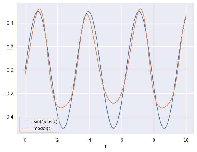
Not bad!
Using automatic differentiation and gradient descent, the neural network weights and biases have been adjusted to make the neural network approximate the function \(\sin(t)\cos(t)\).
It is not perfect, but it gets the general shape.
We could increase the number of epochs to train for longer and improve the accuracy.
PyTorch Primer#
A fully connected network can be created with a few lines in PyTorch (for a similar high-level API in Tensorflow checkout Keras):
torch.manual_seed(123)

net = torch.nn.Sequential(
    torch.nn.Linear(8, 4), #0
    torch.nn.ReLU(),    #1
    torch.nn.Linear(4, 3), #2
    torch.nn.ReLU(),    #3
    torch.nn.Linear(3, 2)  #4
)
As each Linear layer is created, its weight and bias tensors are automatically initialized with random values, so we initially set the torch random seed for reproducible results.
This construction breaks each layer into separate linear and activation “modules”. Each module can be accessed via its index (0-4 in this example):
print(net)
Sequential(
  (0): Linear(in_features=8, out_features=4, bias=True)
  (1): ReLU()
  (2): Linear(in_features=4, out_features=3, bias=True)
  (3): ReLU()
  (4): Linear(in_features=3, out_features=2, bias=True)
)
net[2].weight
Parameter containing:
tensor([[-0.4228, -0.1435, -0.3521,  0.0331],
        [-0.0934, -0.2682, -0.0455,  0.4737],
        [-0.0394,  0.0159, -0.0780,  0.0786]], requires_grad=True)
net[4].bias
Parameter containing:
tensor([0.4928, 0.0345], requires_grad=True)
To run our network in the forward direction, we need some data with the expected number of features (\(D=8\) in this example):
N = 100
D = net[0].in_features
Xin = torch.randn(N, D)
Xout = net(Xin)
The intermediate tensors (\(X_1\), \(\partial\ell/\partial X_1\), …) shown in the data flow diagrams above are usually not preserved, but can be useful to help understand how a network is performing and diagnose problems. To cache these intermediate tensors, use:
trace(net)
Xout = net(Xin)
Each submodule now has input and output attributes:
torch.equal(Xin, net[0].input)
True
torch.equal(net[0].output, net[1].input)
True
Use the verbose option to watch the flow of tensors through the network:
trace(net, verbose=True)
Xout = net(Xin)
0: IN (100, 8) OUT (100, 4)
1: IN (100, 4) OUT (100, 4)
2: IN (100, 4) OUT (100, 3)
3: IN (100, 3) OUT (100, 3)
4: IN (100, 3) OUT (100, 2)
To complete the computational graph we need to calculate a (scalar) loss, for example:
loss = torch.mean(Xout ** 2)
print(loss)
tensor(0.1996, grad_fn=<MeanBackward0>)
We can now back propagate gradients of this loss through the network:
loss.backward()
4: GRAD (100, 2)
3: GRAD (100, 3)
2: GRAD (100, 3)
1: GRAD (100, 4)
0: GRAD (100, 4)
The gradients of each layer’s parameters are now computed and stored, ready to “learn” better parameters through (stochastic) gradient descent (or one of its variants):
net[0].bias.grad
tensor([-0.0285, -0.0276, -0.0335, 0.0646])
Using trace above we have also captured the gradients of the loss with respect to each module’s outputs \(\partial\ell /\partial X_n\):
net[0].output.size(), net[0].grad.size()
(torch.Size([100, 4]), torch.Size([100, 4]))
These gradients can be useful to study since learning of all upstream parameters effectively stops when they become vanishly small (since they multiply those parameter gradients via the chain rule).
Statistical Perspective#
The tensors behind a practical network contain so many values that it is usually not practical to examine them individually. However, we can still gain useful insights if we study their probability distributions.
Build a network to process a large dataset so we have some distributions to study:
torch.manual_seed(123)

N, D = 500, 100
Xin = torch.randn(N, D)

net = torch.nn.Sequential(
    torch.nn.Linear(D, 2 * D),
    torch.nn.Tanh(),
    torch.nn.Linear(2 * D, D),
    torch.nn.ReLU(),
    torch.nn.Linear(D, 10)
)
print(net)
Sequential(
  (0): Linear(in_features=100, out_features=200, bias=True)
  (1): Tanh()
  (2): Linear(in_features=200, out_features=100, bias=True)
  (3): ReLU()
  (4): Linear(in_features=100, out_features=10, bias=True)
)
Note that our network ends with a Linear module instead of an activation, which is typical for regression problems.
Perform forward and backward passes to capture some values:
trace(net, verbose=True)
Xout = net(Xin)
loss = torch.mean(Xout ** 2)
loss.backward()
0: IN (500, 100) OUT (500, 200)
1: IN (500, 200) OUT (500, 200)
2: IN (500, 200) OUT (500, 100)
3: IN (500, 100) OUT (500, 100)
4: IN (500, 100) OUT (500, 10)
4: GRAD (500, 10)
3: GRAD (500, 100)
2: GRAD (500, 100)
1: GRAD (500, 200)
0: GRAD (500, 200)
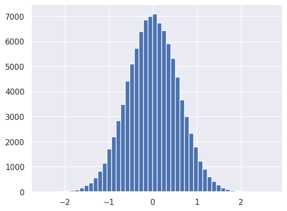
First check that the input to the first module has the expected (unit normal) distribution:
plt.hist(net[0].input.reshape(-1), bins=50);

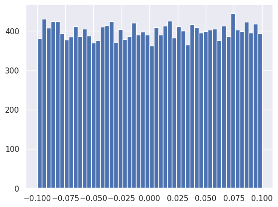
How does torch initialize the parameters (weights and biases) for each layer?
plt.hist(net[0].weight.data.reshape(-1), bins=50);
plt.hist(net[0].bias.data, bins=50);
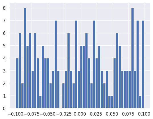
These initial parameter values are sampled from uniform distributions centered on zero with a spread that depends on the number of inputs to the layer:
This default choice is based on empirical studies of image classification problems where the input features (RGB pixel values) were preprocessed to have zero mean and unit variance.
With this choice of weights, the first Linear module mixes up its input values (\(X_0\)) but generally preserves Gaussian shape while slightly reducing its variance (which helps prevent the subsequent activation module from saturating):
plt.hist(net[0].output.reshape(-1), bins=50);
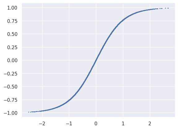
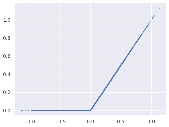
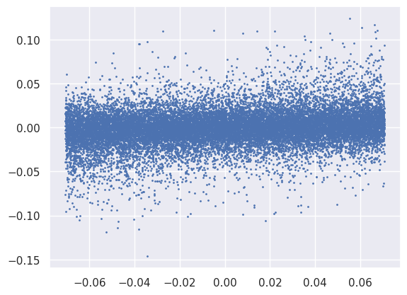
A scatter plot of the the first Tanh activation function’s input and output values just traces out function since it is applied element wise. Note how most of input values do not saturate, which is generally desirable for efficient learning.
plt.scatter(net[1].input.reshape(-1), net[1].output.reshape(-1), s=1);
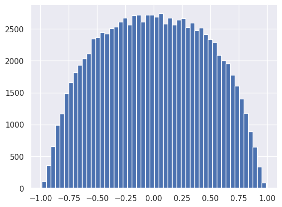
The non-linear activation distorts and clips the output so it no longer resembles a Gaussian:
plt.hist(net[1].output.reshape(-1), bins=50);
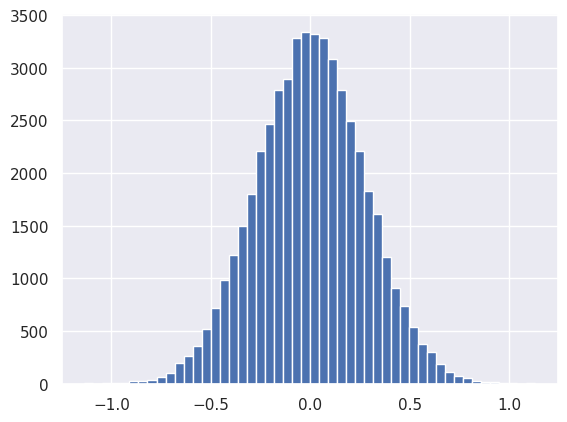
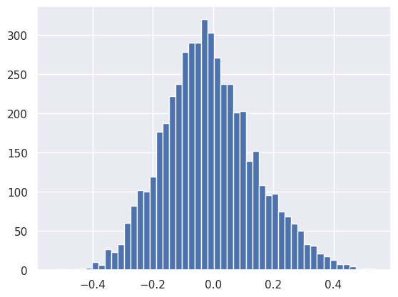
However, the next Linear module restores the Gaussian distribution! How does this happen when neither its inputs nor its parameters have a Gaussian distribution? (Answer: the central limit theorem which we briefly covered earlier).
plt.hist(net[2].output.reshape(-1), bins=50);
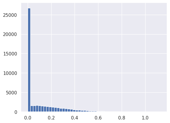
The next activation is ReLU, which effectively piles up all negative values from the previous Linear module into the zero bin:
plt.scatter(net[3].input.reshape(-1), net[3].output.reshape(-1), s=1);
plt.hist(net[3].output.reshape(-1), bins=50);
The final linear layer’s output is again roughly Gaussian, thanks to the central limit theorem:
plt.hist(net[4].output.reshape(-1), bins=50);
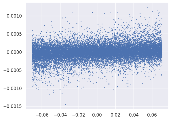
So far we have only looked at distributions of the tensors involved in the forward pass, but there is also a lot to learn from the backwards gradient tensors that we do not have time to delve in to. For example, this scatter plot offers some insight into a suitable learning rate for the second Linear module’s weight parameters:
plt.scatter(net[2].weight.data.reshape(-1), net[2].weight.grad.reshape(-1), s=1);
Note that the normalization of the loss function feeds directly into these gradients, so needs to be considered when setting the learning rate:
Xout = net(Xin)
loss = 100 * torch.mean(Xout ** 2)
loss.backward()
0: IN (500, 100) OUT (500, 200)
1: IN (500, 200) OUT (500, 200)
2: IN (500, 200) OUT (500, 100)
3: IN (500, 100) OUT (500, 100)
4: IN (500, 100) OUT (500, 10)
4: GRAD (500, 10)
3: GRAD (500, 100)
2: GRAD (500, 100)
1: GRAD (500, 200)
0: GRAD (500, 200)
plt.scatter(net[2].weight.data.reshape(-1), net[2].weight.grad.reshape(-1), s=1);
Loss Functions#
In order discover a good set of parameters using optimization, we need to specify a loss function to optimize.
The loss function \(\ell(X_\text{out}, Y_\text{tgt})\) compares the actual network output \(X_\text{out}\) with a corresponding target value \(Y_\text{tgt}\) and approaches some minimum value as their agreement improves.
A loss function must be scalar valued since we need a single gradient for each parameter to implement gradient descent,
Note that the loss normalization is degenerate with the learning rate \(\eta\).
Our choice of loss function is primarily driven by the type of problem we are solving: regression or classification. We introduce the most obvious choices below but there are lots of reasonable variations (see here for the complete PyTorch list).
Regression Loss#
For regression, the \(L_2\) norm is a popular choice,
Optimizing the \(L_2\) norm is equivalent to finding the maximum-likelihood (ML) point estimate for the network parameters (weights and biases) if we assume that the uncertainties in \(Y_\text{tgt}\) are “homoscedastic” (drawn from the same Gaussian distribution).
In PyTorch, the \(L_2\) norm is implemented as torch.nn.MSELoss:
Y = torch.zeros_like(Xout)
loss = torch.nn.MSELoss()(Xout, Y)
In case you actually have a reasonable estimate \(\sigma_Y^i\) of the \(i\)-th sample’s target uncertainty, a better loss function is the \(\chi^2\) statistic:
Binary Classification Loss#
For binary classification problems, the L2 norm can also be used but the binary cross entropy between the target and output probability distributions is often a better choice:
where \(\phi_S\) is the sigmoid (aka logistic) activation function used to coerce arbitrary real values into the range \([0,1]\) required for a probability. An input real value used with sigmoid like this is known as a logit.
The equivalent PyTorch code uses torch.nn.BCELoss:
Xout = torch.ones(10)
Y = torch.zeros(10)
loss = torch.nn.BCELoss()(Xout, Y)
The cross entropy is inspired by information theory and closely related to the KL divergence we met earlier. With this approach, our assumptions are that:
The target values in \(Y_{tgt}\) are all either 0 or 1.
The network output values in \(X_{out}\) are continuous and \(\phi_S(y^{out}_i)\) is interpreted as the corresponding probability that the output is 1.
Note that something like the second assumption is necessary to reconcile the different domains of the data and prediction.
With these assumptions, the likelihood is:
Take a minute to convince yourself that the following expression is equivalent (the case \(\phi_S(X_\text{out}(\Theta)) = Y_\text{tgt} = 0\) requires some care since \(0^0\) is indeterminate):
Using this form, you can show that the cross entropy loss equals the negative-log-likelihood of the \(N\) samples of training data so optimizing BCE is equivalent to finding the ML point estimate of the network parameters under the assumptions above.
For fixed training data, optimizing BCE is also equivalent to minimizing the KL divergence of the network’s predicted discrete probability distribution with respect to the empirical discrete probability distribution of the training data. Therefore, training a binary classification network using the cross-entropy loss is effectively performing a variational inference (VI) to find the network probabilities that are closest to the empirical training probabilities.
Multi-category Classification Loss#
How can we generalize the binary classification cross-entropy loss to problems with more than two categories? The usual approach is to increase the number of output nodes from 1 to the number of categories \(C\), but we can not directly interpret their values as category probabilities since there is no way to ensure that they sum to one. We could simply require that they are all non-negative and renormalize, but a more more robust approach is to convert the vector of output values \(X_\text{out}\) to a corresponding vector of probabilities \(\mathbf{p}\) for category \(j = 1, 2, \ldots, C\) using the softmax function,
which works fine with positive or negative outputs \(X_\text{out}^j\). Note that softmax generalizes the sigmoid function \(\phi_S\) in the following sense:
def softmax(y):
    # subtract out max(y) improve the numerical accuracy
    expy = np.exp(y - np.max(y))
    return expy / expy.sum()
softmax([2, -1, 3])
array([0.26538793, 0.01321289, 0.72139918])
The softmax function effectively implements a winner takes all policy, similar to the sigmoid activation \(\phi_S\), as illustrated in the plot below where:
the color scale indicates, from left to right, \(p_1, p_2\) and \(p_3\) for three categories,
\(y_1\) and \(y_2\) are varied over the same range, and
\(y_3\) is fixed to the middle of this range.
def plot_softmax(ylo, yhi, n=100):
    y_grid = np.linspace(ylo, yhi, n)
    y3 = 0.5 * (ylo + yhi)
    p_grid = np.array([softmax([y1, y2, y3]) for y1 in y_grid for y2 in y_grid]).reshape(n, n, 3)
    _, ax = plt.subplots(1, 3, figsize=(10.5, 3))
    for k in range(3):
        ax[k].imshow(p_grid[:, :, k], interpolation='none', origin='lower', extent=[ylo, yhi, ylo, yhi])
        ax[k].set_xlabel('$y_1$')
        ax[k].set_ylabel('$y_2$')
        if k != 0: ax[k].axvline(y3, c='gray', ls='--')
        if k != 1: ax[k].axhline(y3, c='gray', ls='--')
        if k != 2: ax[k].plot([ylo, yhi], [ylo, yhi], c='gray', ls='--')
        ax[k].grid(False)

plot_softmax(0, 15)
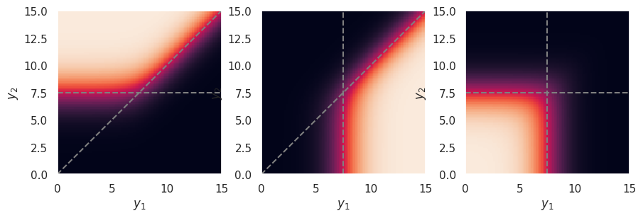
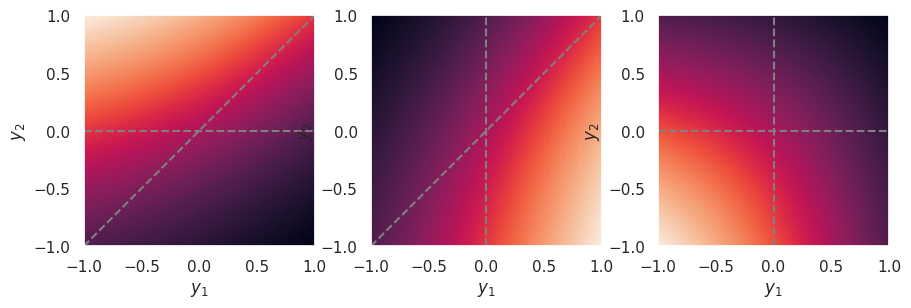
The example above assumed output activations that can be large and positive, such as relu or elu. However, the strength of the winner takes all effect depends on how the outputs are scaled, and is relatively weak for output activations that saturate on both sides, such as sigmoid or tanh, which is why these are generally not used for classification outputs:
plot_softmax(-1, +1)
Note that we assume one-hot encoding of the vector target values \(\mathbf{y}^{out}\), which is not very efficient (unless using sparse-optimized data structures) compared to a single integer target value \(y^{train} = 0, 1, \ldots, C-1\). However, sklearn has a convenient utility to convert integers to one-hot encoded vectors (use sparse=True to return vectors in an efficient scipy sparse array).
Acknowledgments#
Initial version: Mark Neubauer
© Copyright 2026