Unsupervised Learning and Anomaly Detection

%matplotlib inline
import matplotlib.pyplot as plt
import seaborn as sns; sns.set_theme()
import numpy as np
import pandas as pd
import os.path
import subprocess
import matplotlib.collections
import scipy.signal
from sklearn import model_selection
import warnings
warnings.filterwarnings('ignore')

import torch
import copy
from pylab import rcParams
from matplotlib import rc
from sklearn.model_selection import train_test_split
from torch import nn, optim
import torch.nn.functional as F
from scipy.io import arff

RANDOM_SEED = 42
np.random.seed(RANDOM_SEED)
torch.manual_seed(RANDOM_SEED)

<torch._C.Generator at 0x134200410>

Helpers for Getting, Loading, and Locating Data

def wget_data(url: str, local_path='./tmp_data'):
  os.makedirs(local_path, exist_ok=True)

  p = subprocess.Popen(["wget", "-nc", "-P", local_path, url], stderr=subprocess.PIPE, encoding='UTF-8')
  rc = None

  while rc is None:
    line = p.stderr.readline().strip('\n')
    if len(line) > 0:
      print(line)
    rc = p.poll()

def locate_data(name, check_exists=True):
    local_path='./tmp_data'
    path = os.path.join(local_path, name)
    if check_exists and not os.path.exists(path):
        raise RuxntimeError('No such data file: {}'.format(path))
    return path

Get Data

wget_data('https://raw.githubusercontent.com/illinois-mlp/MachineLearningForPhysics/main/data/ECG5000_TRAIN.arff')
wget_data('https://raw.githubusercontent.com/illinois-mlp/MachineLearningForPhysics/main/data/ECG5000_TEST.arff')

File ‘./tmp_data/ECG5000_TRAIN.arff’ already there; not retrieving.
File ‘./tmp_data/ECG5000_TEST.arff’ already there; not retrieving.

Networks for Unsupervised Learning

Neural networks are usually used for supervised learning since their learning is accomplished by optimizing a loss function that compares the network’s outputs with some target values. However, it is possible to perform unsupervised learning if we can somehow use the same data for both the input values and the target output values. This requires that the network have the same number of input and output nodes, and effectively means that we are asking it to learn the identify function, which does not sound obviously useful.

Suppose we have a single hidden layer with the same number of nodes as the input and output layers, then all the network has to do is pass each input value through to the output, which does not require any training at all! However, if the hidden layer has fewer nodes then we are asking the network to solve a more interesting problem: how can the input dataset be encoded and then decoded. This is the same dimensionality reduction problem we discussed earlier, and is known as an autoencoder network as we covered in the AutoEncoders notebook since it learns to encode itself:

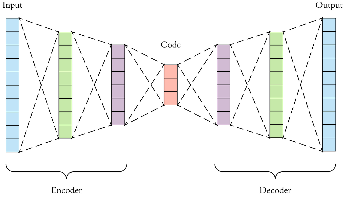
The network can be thought of as the combination of separate encoder and decoder networks, with the encoder feeding its output latent variables \(\mathbf{z}\) into the decoder. Although the architecture looks symmetric, the encoder and decoder will generally learn different parameters because of the asymmetry introduced by nonlinear activations. The figure represents a high-level design pattern and the internal architectures of the encoder and decoder networks should be customized for the type of data being encoded (and typically combined convolutional and dense layers).

Example: Time Series Anomaly Detection using LSTM Autoencoders

In this example, we will learn to:

• Prepare a dataset for Anomaly Detection from Time Series Data

• Build an LSTM Autoencoder with PyTorch

• Train and evaluate your model

• Choose a threshold for anomaly detection

• Classify unseen examples as normal or anomaly

While our Time Series data is univariate (we have only 1 feature), the code should work for multivariate datasets (multiple features) with little or no modification. Feel free to try it!

Brief LSTM Review

A Long Short-Term Memory (LSTM) is a type of Recurrent Neural Network (RNN) designed to handle long-term dependencies in sequential data, such as text, time series, and speech. LSTMs are known for their ability to mitigate the vanishing gradient problem that plagues standard RNNs, allowing them to learn and remember information over longer sequences of data.

Key Features of LSTMs:

• Memory Cell: LSTMs introduce a memory cell that acts as a “memory” for the network, allowing it to store and retrieve information over time.

• Gates: LSTMs use “gates” (input, forget, and output gates) to control the flow of information into, out of, and within the memory cell.

• Vanishing Gradient Problem: LSTMs are designed to prevent the gradients from vanishing or exploding as they propagate through the network over time, making them more effective for learning long-term relationships in sequential data.

• Sequence Learning: LSTMs are particularly well-suited for tasks that involve processing sequential data, such as natural language processing (language modeling, machine translation), speech recognition, and time series forecasting.

How LSTMs Work:

1. Input: The LSTM receives an input sequence, where each input represents a time step.

2. Gates: The gates regulate the flow of information into the memory cell and the output from the cell.

3. Memory Cell: The memory cell stores and updates its internal state based on the input and the previous state.

4. Output: The LSTM produces an output at each time step based on the current cell state and the input.

Advantages of LSTMs:

• Long-term dependencies: LSTMs are capable of learning long-term dependencies in sequential data.

• Vanishing gradient problem: LSTMs mitigate the vanishing gradient problem, making them more effective for processing long sequences.

• Wide range of applications: LSTMs have been successfully applied to many sequence learning tasks.

Data

The dataset contains 5,000 Time Series examples (obtained with ECG) with 140 timesteps. Each sequence corresponds to a single heartbeat from a single patient with congestive heart failure.

An electrocardiogram (ECG or EKG) is a test that checks how your heart is functioning by measuring the electrical activity of the heart. It measures the electrical activity of your heart. It uses small electrodes attached to your skin to detect the tiny electrical signals that control your heartbeat. With each heart beat, an electrical impulse (or wave) travels through your heart. This wave causes the muscle to squeeze and pump blood from the heart. Source

• What it measures: An ECG records the electrical impulses that cause your heart to beat, showing how the signals travel through your heart’s chambers.

• How it’s done: During an ECG, electrodes are attached to your chest, arms, and legs using adhesive patches or small suction cups.

• What it shows: The ECG produces a graphical representation of your heart’s electrical activity, known as an ECG tracing.

• Why it’s used: ECGs are used to diagnose and monitor various heart conditions, including arrhythmias, coronary artery disease, heart attacks, and heart failure.

• What it can reveal: An ECG can help doctors detect changes in heart rate, rhythm, and electrical conduction, which may indicate a heart problem.

We have 5 types of hearbeats (classes):

• Normal (N)

• R-on-T Premature Ventricular Contraction (R-on-T PVC)

• Premature Ventricular Contraction (PVC)

• Supra-ventricular Premature or Ectopic Beat (SP or EB)

• Unclassified Beat (UB).

Assuming a healthy heart and a typical rate of 70 to 75 beats per minute, each cardiac cycle, or heartbeat, takes about 0.8 seconds to complete the cycle. Frequency: 60–100 per minute (Humans) Duration: 0.6–1 second (Humans) Source

device = torch.device("cuda" if torch.cuda.is_available() else "cpu")
print(device)

cpu

The data comes in multiple formats. We’ll load the arff files into Pandas data frames:

with open(locate_data('ECG5000_TRAIN.arff')) as f:
  data, meta = arff.loadarff(f)
  train = pd.DataFrame(data)
  print(train.shape)

with open(locate_data('ECG5000_TEST.arff')) as f:
  data, meta = arff.loadarff(f)
  test = pd.DataFrame(data)
  print(test.shape)

(500, 141)
(4500, 141)

We’ll combine the training and test data into a single data frame. This will give us more data to train our Autoencoder. We’ll also shuffle it:

df = pd.concat([train, test])
df = df.sample(frac=1.0)
df.shape

(5000, 141)

df.head()

	att1	att2	att3	att4	att5	att6	att7	att8	att9	att10	...	att132	att133	att134	att135	att136	att137	att138	att139	att140	target
1001	1.469756	-1.048520	-3.394356	-4.254399	-4.162834	-3.822570	-3.003609	-1.799773	-1.500033	-1.025095	...	0.945178	1.275588	1.617218	1.580279	1.306195	1.351674	1.915517	1.672103	-1.039932	b'1'
2086	-1.998602	-3.770552	-4.267091	-4.256133	-3.515288	-2.554540	-1.699639	-1.566366	-1.038815	-0.425483	...	1.008577	1.024698	1.051141	1.015352	0.988475	1.050191	1.089509	1.465382	0.799517	b'1'
2153	-1.187772	-3.365038	-3.695653	-4.094781	-3.992549	-3.425381	-2.057643	-1.277729	-1.307397	-0.623098	...	1.085007	1.467196	1.413850	1.283822	0.923126	0.759235	0.932364	1.216265	-0.824489	b'1'
555	0.604969	-1.671363	-3.236131	-3.966465	-4.067820	-3.551897	-2.582864	-1.804755	-1.688151	-1.025897	...	0.545222	0.649363	0.986846	1.234495	1.280039	1.215985	1.617971	2.196543	0.023843	b'1'
205	-1.197203	-3.270123	-3.778723	-3.977574	-3.405060	-2.392634	-1.726322	-1.572748	-0.920075	-0.388731	...	0.828168	0.914338	1.063077	1.393479	1.469756	1.392281	1.144732	1.668263	1.734676	b'1'

5 rows × 141 columns

We have 5,000 examples. Each row represents a single heartbeat record. Let’s name the possible classes:

CLASS_NORMAL = 1
#class_names = ['Normal','R on T','PVC','SP','UB'] # This ordering sometimes produces wrong counts histogram. Need to check if it affects plots that use class_names
class_names = ['Normal','PVC','R on T','SP','UB']

Next, we’ll rename the last column to target, so its easier to reference it:

new_columns = list(df.columns)
new_columns[-1] = 'target'
df.columns = new_columns

Exploratory Data Analysis

Let’s check how many examples for each heartbeat class do we have:

df.target.value_counts()

target
b'1'    2919
b'2'    1767
b'4'     194
b'3'      96
b'5'      24
Name: count, dtype: int64

Let’s plot the results:

ax = sns.countplot(x=df.target, data=df)
ax.set_xticklabels(class_names)
plt.show()

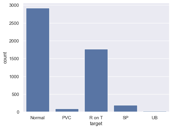
The normal class, has by far, the most examples. This is great because we’ll use it to train our model.

Let’s have a look at an averaged (smoothed out with one standard deviation on top and bottom of it) Time Series for each class:

def plot_time_series_class(data, class_name, ax, n_steps=10):
  time_series_df = pd.DataFrame(data)

  smooth_path = time_series_df.rolling(n_steps).mean()
  path_deviation = 2 * time_series_df.rolling(n_steps).std()

  under_line = (smooth_path - path_deviation)[0]
  over_line = (smooth_path + path_deviation)[0]

  ax.plot(smooth_path, linewidth=2)
  ax.fill_between(
    path_deviation.index,
    under_line,
    over_line,
    alpha=.125
  )
  ax.set_title(class_name)

classes = df.target.unique()

fig, axs = plt.subplots(
  nrows=len(classes) // 3 + 1,
  ncols=3,
  sharey=True,
  figsize=(14, 8)
)

for i, cls in enumerate(classes):
  ax = axs.flat[i]
  data = df[df.target == cls] \
    .drop(labels='target', axis=1) \
    .mean(axis=0) \
    .to_numpy()
  plot_time_series_class(data, class_names[i], ax)

fig.delaxes(axs.flat[-1])
fig.tight_layout();

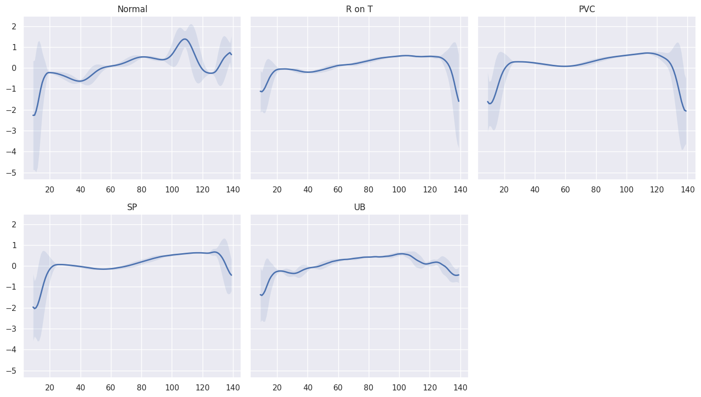
It is very good that the normal class has a distinctly different pattern than all other classes. Maybe our model will be able to detect anomalies?

LSTM Autoencoder

The Autoencoder’s job is to get some input data, pass it through the model, and obtain a reconstruction of the input. The reconstruction should match the input as much as possible. The trick is to use a small number of parameters, so your model learns a compressed representation of the data.

In a sense, Autoencoders try to learn only the most important features (compressed version) of the data. Here, we’ll have a look at how to feed Time Series data to an Autoencoder. We’ll use a couple of LSTM layers (hence the LSTM Autoencoder) to capture the temporal dependencies of the data.

To classify a sequence as normal or an anomaly, we’ll pick a threshold above which a heartbeat is considered abnormal.

Reconstruction Loss

When training an Autoencoder, the objective is to reconstruct the input as best as possible. This is done by minimizing a loss function (just like in supervised learning). This function is known as reconstruction loss. Cross-entropy loss and Mean squared error are common examples.

Anomaly Detection in ECG Data

We’ll use normal heartbeats as training data for our model and record the reconstruction loss. But first, we need to prepare the data:

Data Preprocessing

Let’s get all normal heartbeats and drop the target (class) column:

normal_df = df[df.target == str(CLASS_NORMAL).encode('utf-8')].drop(labels='target', axis=1)
normal_df.shape

(2919, 140)

We’ll merge all other classes and mark them as anomalies:

anomaly_df = df[df.target != str(CLASS_NORMAL).encode('utf-8')].drop(labels='target', axis=1)
anomaly_df.shape

(2081, 140)

We’ll split the normal examples into train, validation and test sets:

train_df, val_df = train_test_split(
  normal_df,
  test_size=0.15,
  random_state=RANDOM_SEED
)

val_df, test_df = train_test_split(
  val_df,
  test_size=0.33,
  random_state=RANDOM_SEED
)

We need to convert our examples into tensors, so we can use them to train our Autoencoder. Let’s write a helper function for that:

def create_dataset(df):

  sequences = df.astype(np.float32).to_numpy().tolist()

  dataset = [torch.tensor(s).unsqueeze(1).float() for s in sequences]

  n_seq, seq_len, n_features = torch.stack(dataset).shape

  return dataset, seq_len, n_features

Each Time Series will be converted to a 2D Tensor in the shape sequence length x number of features (140x1 in our case).

Let’s create some datasets:

train_dataset, seq_len, n_features = create_dataset(train_df)
val_dataset, _, _ = create_dataset(val_df)
test_normal_dataset, _, _ = create_dataset(test_df)
test_anomaly_dataset, _, _ = create_dataset(anomaly_df)

LSTM Autoencoder

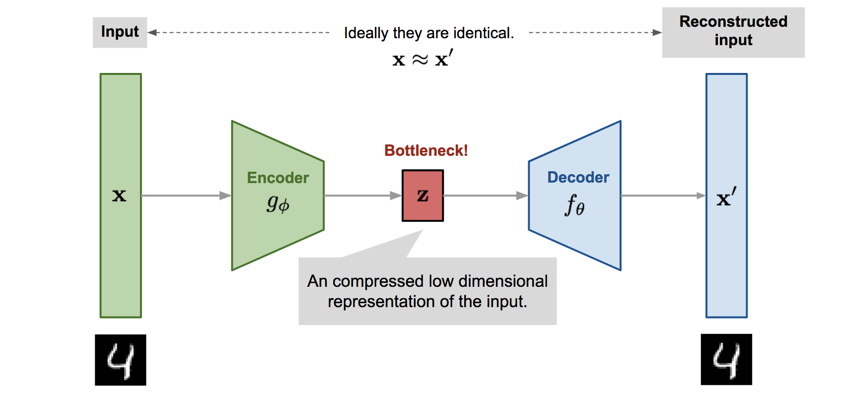
Sample Autoencoder Architecture Image Source

The general Autoencoder architecture consists of two components. An Encoder that compresses the input and a Decoder that tries to reconstruct it.

We’ll use the LSTM Autoencoder from this GitHub repo with some small tweaks. Our model’s job is to reconstruct Time Series data. Let’s start with the Encoder:

class Encoder(nn.Module):

  def __init__(self, seq_len, n_features, embedding_dim=64):
    super(Encoder, self).__init__()

    self.seq_len, self.n_features = seq_len, n_features
    self.embedding_dim, self.hidden_dim = embedding_dim, 2 * embedding_dim

    self.rnn1 = nn.LSTM(
      input_size=n_features,
      hidden_size=self.hidden_dim,
      num_layers=1,
      batch_first=True
    )

    self.rnn2 = nn.LSTM(
      input_size=self.hidden_dim,
      hidden_size=embedding_dim,
      num_layers=1,
      batch_first=True
    )

  def forward(self, x):
    x = x.reshape((1, self.seq_len, self.n_features))

    x, (_, _) = self.rnn1(x)
    x, (hidden_n, _) = self.rnn2(x)

    return hidden_n.reshape((self.n_features, self.embedding_dim))

The Encoder uses two LSTM layers to compress the Time Series data input.

Next, we’ll decode the compressed representation using a Decoder:

class Decoder(nn.Module):

  def __init__(self, seq_len, input_dim=64, n_features=1):
    super(Decoder, self).__init__()

    self.seq_len, self.input_dim = seq_len, input_dim
    self.hidden_dim, self.n_features = 2 * input_dim, n_features

    self.rnn1 = nn.LSTM(
      input_size=input_dim,
      hidden_size=input_dim,
      num_layers=1,
      batch_first=True
    )

    self.rnn2 = nn.LSTM(
      input_size=input_dim,
      hidden_size=self.hidden_dim,
      num_layers=1,
      batch_first=True
    )

    self.output_layer = nn.Linear(self.hidden_dim, n_features)

  def forward(self, x):
    x = x.repeat(self.seq_len, self.n_features)
    x = x.reshape((self.n_features, self.seq_len, self.input_dim))

    x, (hidden_n, cell_n) = self.rnn1(x)
    x, (hidden_n, cell_n) = self.rnn2(x)
    x = x.reshape((self.seq_len, self.hidden_dim))

    return self.output_layer(x)

Our Decoder contains two LSTM layers and an output layer that gives the final reconstruction.

Time to wrap everything into an easy to use module:

class RecurrentAutoencoder(nn.Module):

  def __init__(self, seq_len, n_features, embedding_dim=64):
    super(RecurrentAutoencoder, self).__init__()

    self.encoder = Encoder(seq_len, n_features, embedding_dim).to(device)
    self.decoder = Decoder(seq_len, embedding_dim, n_features).to(device)

  def forward(self, x):
    x = self.encoder(x)
    x = self.decoder(x)

    return x

Our Autoencoder passes the input through the Encoder and Decoder. Let’s create an instance of it:

model = RecurrentAutoencoder(seq_len, n_features, 128)
model = model.to(device)

Training

Let’s write a helper function for our training process:

def train_model(model, train_dataset, val_dataset, n_epochs):
  optimizer = torch.optim.Adam(model.parameters(), lr=1e-3)
  criterion = nn.L1Loss(reduction='sum').to(device)
  history = dict(train=[], val=[])

  best_model_wts = copy.deepcopy(model.state_dict())
  best_loss = 10000.0

  for epoch in range(1, n_epochs + 1):
    model = model.train()

    train_losses = []
    for seq_true in train_dataset:
      optimizer.zero_grad()

      seq_true = seq_true.to(device)
      seq_pred = model(seq_true)

      loss = criterion(seq_pred, seq_true)

      loss.backward()
      optimizer.step()

      train_losses.append(loss.item())

    val_losses = []
    model = model.eval()
    with torch.no_grad():
      for seq_true in val_dataset:

        seq_true = seq_true.to(device)
        seq_pred = model(seq_true)

        loss = criterion(seq_pred, seq_true)
        val_losses.append(loss.item())

    train_loss = np.mean(train_losses)
    val_loss = np.mean(val_losses)

    history['train'].append(train_loss)
    history['val'].append(val_loss)

    if val_loss < best_loss:
      best_loss = val_loss
      best_model_wts = copy.deepcopy(model.state_dict())

    print(f'Epoch {epoch}: train loss {train_loss} val loss {val_loss}')

  model.load_state_dict(best_model_wts)
  return model.eval(), history

At each epoch, the training process feeds our model with all training examples and evaluates the performance on the validation set. Note that we’re using a batch size of 1 (our model sees only 1 sequence at a time). We also record the training and validation set losses during the process.

Note that we’re minimizing the L1Loss, which measures the MAE (mean absolute error). Why? The reconstructions seem to be better than with MSE (mean squared error).

We’ll get the version of the model with the smallest validation error. Let’s do some training:

model, history = train_model(
  model,
  train_dataset,
  val_dataset,
  n_epochs=150
)

Epoch 1: train loss 70.19056519843167 val loss 55.545283333840224
Epoch 2: train loss 57.20439573393287 val loss 53.2183632053206
Epoch 3: train loss 53.80251925667175 val loss 51.787326721608025
Epoch 4: train loss 53.50249311915332 val loss 52.1923034850241
Epoch 5: train loss 51.639859836459976 val loss 50.23866700312384
Epoch 6: train loss 47.88762839923506 val loss 53.42915126813556
Epoch 7: train loss 44.5796035203853 val loss 42.75591913425068
Epoch 8: train loss 43.05668973250045 val loss 41.69073425136735
Epoch 9: train loss 36.804902854344384 val loss 28.941658182762588
Epoch 10: train loss 29.600385176948077 val loss 27.772434221599696
Epoch 11: train loss 29.258839591478733 val loss 33.79314185002558
Epoch 12: train loss 27.309336170271873 val loss 29.403204198583403
Epoch 13: train loss 26.56631477529702 val loss 25.562526377394743
Epoch 14: train loss 25.581571012771402 val loss 26.178377704815652
Epoch 15: train loss 24.73337686278079 val loss 28.74295396772261
Epoch 16: train loss 23.183967294735275 val loss 29.078925552628554
Epoch 17: train loss 23.142798073202407 val loss 21.02237903542893
Epoch 18: train loss 21.924223153738186 val loss 24.21762883052891
Epoch 19: train loss 21.104562202416712 val loss 20.23192710030201
Epoch 20: train loss 20.47691583152934 val loss 22.912674659755044
Epoch 21: train loss 20.040546160078684 val loss 18.938482645835485
Epoch 22: train loss 19.584992215019327 val loss 18.982437735938376
Epoch 23: train loss 19.018079930666424 val loss 20.806668545198928
Epoch 24: train loss 18.504388450567205 val loss 18.30796128491086
Epoch 25: train loss 18.096634402384637 val loss 19.596596021294186
Epoch 26: train loss 17.977364436698892 val loss 16.531875984660594
Epoch 27: train loss 17.49705117597353 val loss 18.28265956318826
Epoch 28: train loss 18.026098470253505 val loss 17.385052781869934
Epoch 29: train loss 17.374587030191663 val loss 18.157290784165316
Epoch 30: train loss 17.16383284534576 val loss 17.862681655753594
Epoch 31: train loss 16.66365962564729 val loss 15.49548804312436
Epoch 32: train loss 16.405945794229687 val loss 18.52142742143963
Epoch 33: train loss 16.062661001058608 val loss 14.830465095441904
Epoch 34: train loss 16.47399080707776 val loss 17.471961138598342
Epoch 35: train loss 15.997433853456927 val loss 15.624564058544692
Epoch 36: train loss 15.45416613021045 val loss 13.819568647052648
Epoch 37: train loss 15.674591416363176 val loss 15.529796063289707
Epoch 38: train loss 15.053373992947598 val loss 15.9429453696814
Epoch 39: train loss 15.373062103998752 val loss 15.99911313496352
Epoch 40: train loss 14.997124674242382 val loss 16.14874661090838
Epoch 41: train loss 14.78773114374692 val loss 15.053109400101489
Epoch 42: train loss 14.707472309187889 val loss 13.474772160370602
Epoch 43: train loss 14.391030698474113 val loss 16.305593604520727
Epoch 44: train loss 14.542153571219947 val loss 15.953227477675819
Epoch 45: train loss 15.172505170575365 val loss 13.980109895048695
Epoch 46: train loss 14.188497360749189 val loss 12.644973229222737
Epoch 47: train loss 14.156689580819723 val loss 21.353175908632245
Epoch 48: train loss 50.04139142169053 val loss 49.17329901477176
Epoch 49: train loss 46.201949142246946 val loss 43.659058691291676
Epoch 50: train loss 42.91428000155306 val loss 43.057076444398014
Epoch 51: train loss 41.81053997364221 val loss 41.106021588166016
Epoch 52: train loss 36.06166249520833 val loss 39.88905889100996
Epoch 53: train loss 29.183639168499074 val loss 26.974961004159557
Epoch 54: train loss 26.367558816420075 val loss 27.51501340508054
Epoch 55: train loss 26.53801757123671 val loss 39.89739027446447
Epoch 56: train loss 39.92649830161252 val loss 41.40678741663389
Epoch 57: train loss 35.69660516690458 val loss 29.03401455537451
Epoch 58: train loss 25.09197178486613 val loss 20.72612377401098
Epoch 59: train loss 23.13466597545152 val loss 18.418487984979517
Epoch 60: train loss 21.964455101193078 val loss 20.055133132804375
Epoch 61: train loss 40.05612799372706 val loss 37.54572868347168
Epoch 62: train loss 39.15776094146815 val loss 38.9643552929875
Epoch 63: train loss 38.448927825903134 val loss 35.390615183338774
Epoch 64: train loss 37.809167015509274 val loss 39.99620886141936
Epoch 65: train loss 34.09364483328608 val loss 27.30450067747982
Epoch 66: train loss 26.67849037619379 val loss 20.352936210892715
Epoch 67: train loss 24.84206325188129 val loss 33.320356661956055
Epoch 68: train loss 34.431856618586785 val loss 32.346698956278
Epoch 69: train loss 30.98668835096809 val loss 26.43371902960559
Epoch 70: train loss 26.04953423799502 val loss 24.974476687330434
Epoch 71: train loss 23.299769980058898 val loss 20.337625868084487
Epoch 72: train loss 21.48273552352985 val loss 18.126675771771843
Epoch 73: train loss 20.842392928366795 val loss 21.02987113991695
Epoch 74: train loss 20.490705648865827 val loss 20.880575531578714
Epoch 75: train loss 20.557456831065267 val loss 22.441138277281674
Epoch 76: train loss 20.451879095425774 val loss 35.61199761087984
Epoch 77: train loss 20.20753402740712 val loss 19.251601261490443
Epoch 78: train loss 19.92655499065081 val loss 20.376938081031774
Epoch 79: train loss 20.20205936293504 val loss 20.11863258348797
Epoch 80: train loss 19.13581985737325 val loss 17.33350148380006
Epoch 81: train loss 19.631320482105654 val loss 18.23948536960745
Epoch 82: train loss 19.085387102493783 val loss 22.58678812866732
Epoch 83: train loss 19.56715456567816 val loss 16.282159437498542
Epoch 84: train loss 18.86151957117901 val loss 22.12527833294136
Epoch 85: train loss 19.182493048778998 val loss 15.719699169588576
Epoch 86: train loss 18.786777692185154 val loss 15.68992683098178
Epoch 87: train loss 18.78033543017448 val loss 23.52071121528287
Epoch 88: train loss 18.26201426930026 val loss 18.25598847906744
Epoch 89: train loss 18.979437475769522 val loss 21.100039452822948
Epoch 90: train loss 18.26648298361185 val loss 19.28377089972382
Epoch 91: train loss 18.31599943064144 val loss 24.22523792449118
Epoch 92: train loss 18.298746783230776 val loss 28.706830978393555
Epoch 93: train loss 19.08678672833579 val loss 15.865922319197411
Epoch 94: train loss 18.08626968233108 val loss 23.420287727902775
Epoch 95: train loss 17.652017629900943 val loss 15.142815327888462
Epoch 96: train loss 18.181185933189592 val loss 25.33449844776974
Epoch 97: train loss 17.877270106969462 val loss 33.13134558615831
Epoch 98: train loss 17.836640245921185 val loss 15.37667643739095
Epoch 99: train loss 16.938111701351843 val loss 16.563636779785156
Epoch 100: train loss 17.732364453312275 val loss 14.672442454119999
Epoch 101: train loss 17.263540312341508 val loss 15.82090921532172
Epoch 102: train loss 16.891706773418903 val loss 16.7379050905794
Epoch 103: train loss 17.13709879594193 val loss 14.146806155455398
Epoch 104: train loss 16.764518058189505 val loss 19.440087813159305
Epoch 105: train loss 16.94334373873888 val loss 15.222742149040561
Epoch 106: train loss 16.183697756237198 val loss 13.306550038959386
Epoch 107: train loss 16.64517932262982 val loss 16.13168755488998
Epoch 108: train loss 16.37091232739548 val loss 14.694227990030022
Epoch 109: train loss 16.702855778624578 val loss 15.194658243615473
Epoch 110: train loss 16.91737700296669 val loss 15.045723869532042
Epoch 111: train loss 16.59945496970826 val loss 19.52368563759449
Epoch 112: train loss 16.260910302484675 val loss 16.171519328302896
Epoch 113: train loss 15.8463382732479 val loss 14.829655901157002
Epoch 114: train loss 16.28005094059241 val loss 16.68857728580566
Epoch 115: train loss 15.451319722195201 val loss 14.870933399265537
Epoch 116: train loss 15.672055015348706 val loss 13.178509814747365
Epoch 117: train loss 16.393067020122587 val loss 14.099442119077612
Epoch 118: train loss 15.825646905925955 val loss 13.307889482673932
Epoch 119: train loss 15.71289432418774 val loss 14.201728811036197
Epoch 120: train loss 15.860002806570106 val loss 13.228547328975013
Epoch 121: train loss 15.53800718537361 val loss 13.781301809252325
Epoch 122: train loss 15.34830952939945 val loss 13.269842797171947
Epoch 123: train loss 15.222065412820418 val loss 13.787556535961684
Epoch 124: train loss 15.34281487851218 val loss 22.795164147334702
Epoch 125: train loss 15.242534686076645 val loss 15.581529978599157
Epoch 126: train loss 14.984672280580273 val loss 13.194535392136297
Epoch 127: train loss 14.719113676262594 val loss 16.74072455383405
Epoch 128: train loss 14.400070794115909 val loss 14.215379734494988
Epoch 129: train loss 14.55763864036723 val loss 13.726758979693209
Epoch 130: train loss 14.519240352618315 val loss 12.753542180761135
Epoch 131: train loss 14.505081076816127 val loss 13.40780791324967
Epoch 132: train loss 14.800157288686252 val loss 12.927813090562006
Epoch 133: train loss 14.541326379257073 val loss 13.011886248409544
Epoch 134: train loss 14.405127430577185 val loss 12.052384399309908
Epoch 135: train loss 14.595999834759493 val loss 22.06686915960735
Epoch 136: train loss 14.226204098928653 val loss 12.305029219734791
Epoch 137: train loss 14.080185916144153 val loss 12.431378122075833
Epoch 138: train loss 14.08342739594939 val loss 12.217355282233436
Epoch 139: train loss 13.97979081998377 val loss 12.693149750550045
Epoch 140: train loss 13.63878089235176 val loss 12.318664846973615
Epoch 141: train loss 13.919130394315586 val loss 15.256824709856469
Epoch 142: train loss 16.13320877954682 val loss 17.077763248222272
Epoch 143: train loss 15.087361056686456 val loss 15.29185129107062
Epoch 144: train loss 14.432223819715754 val loss 12.79300432888721
Epoch 145: train loss 14.343365429390442 val loss 12.252096006894682
Epoch 146: train loss 13.892574746202241 val loss 13.744810376151023
Epoch 147: train loss 13.876122432002997 val loss 12.75807917891102
Epoch 148: train loss 13.617831775998935 val loss 12.758630116238121
Epoch 149: train loss 13.805896500145797 val loss 14.246482142816225
Epoch 150: train loss 13.779111992491199 val loss 15.29199789001673

ax = plt.figure().gca()

ax.plot(history['train'])
ax.plot(history['val'])
plt.ylabel('Loss')
plt.xlabel('Epoch')
plt.legend(['train', 'test'])
plt.title('Loss over training epochs')
plt.show();

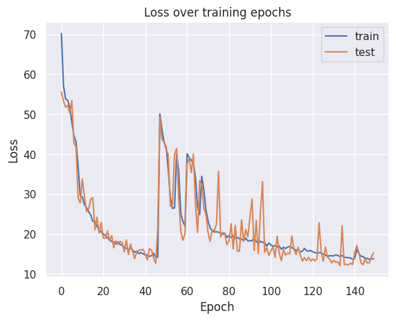
Our model converged quite well. Seems like we might’ve needed a larger validation set to smoothen the results, but that’ll do for now.

Saving the Model

Let’s store the model for later use:

MODEL_PATH = 'model.pth'

torch.save(model, MODEL_PATH)

Uncomment the next lines, if you want to download and load the pre-trained model:

# !gdown --id 1jEYx5wGsb7Ix8cZAw3l5p5pOwHs3_I9A
# model = torch.load('model.pth')
# model = model.to(device)

Choosing a Threshold

With our model at hand, we can have a look at the reconstruction error on the training set. Let’s start by writing a helper function to get predictions from our model:

def predict(model, dataset):
  predictions, losses = [], []
  criterion = nn.L1Loss(reduction='sum').to(device)
  with torch.no_grad():
    model = model.eval()
    for seq_true in dataset:
      seq_true = seq_true.to(device)
      seq_pred = model(seq_true)

      loss = criterion(seq_pred, seq_true)

      predictions.append(seq_pred.cpu().numpy().flatten())
      losses.append(loss.item())
  return predictions, losses

Our function goes through each example in the dataset and records the predictions and losses. Let’s get the losses and have a look at them:

_, losses = predict(model, train_dataset)

sns.distplot(losses, bins=50, kde=True);

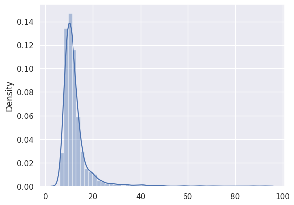
THRESHOLD = 26

Evaluation

Using the threshold, we can turn the problem into a simple binary classification task:

• If the reconstruction loss for an example is below the threshold, we’ll classify it as a normal heartbeat

• Alternatively, if the loss is higher than the threshold, we’ll classify it as an anomaly

Normal Heartbeats

Let’s check how well our model does on normal heartbeats. We’ll use the normal heartbeats from the test set (our model haven’t seen those):

predictions, pred_losses = predict(model, test_normal_dataset)
sns.distplot(pred_losses, bins=50, kde=True);

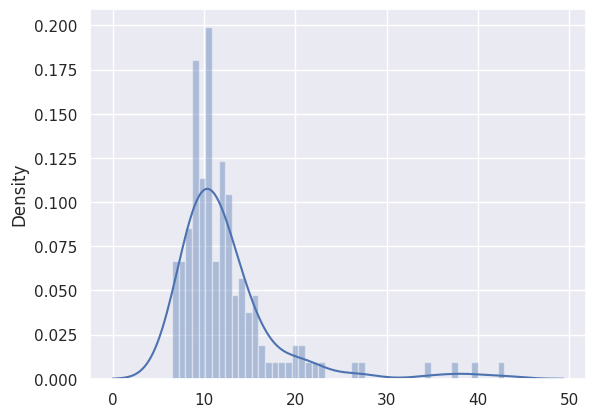
We’ll count the correct predictions:

correct = sum(l <= THRESHOLD for l in pred_losses)
print(f'Correct normal predictions: {correct}/{len(test_normal_dataset)}')

Correct normal predictions: 139/145

Anomalies

We’ll do the same with the anomaly examples, but their number is much higher. We’ll get a subset that has the same size as the normal heartbeats:

anomaly_dataset = test_anomaly_dataset[:len(test_normal_dataset)]

Now we can take the predictions of our model for the subset of anomalies:

predictions, pred_losses = predict(model, anomaly_dataset)
sns.distplot(pred_losses, bins=50, kde=True);

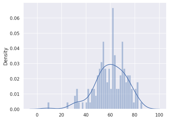
Finally, we can count the number of examples above the threshold (considered as anomalies):

correct = sum(l > THRESHOLD for l in pred_losses)
print(f'Correct anomaly predictions: {correct}/{len(anomaly_dataset)}')

Correct anomaly predictions: 143/145

We have very good results. In the real world, you can tweak the threshold depending on what kind of errors you want to tolerate. In this case, you might want to have more false positives (normal heartbeats considered as anomalies) than false negatives (anomalies considered as normal).

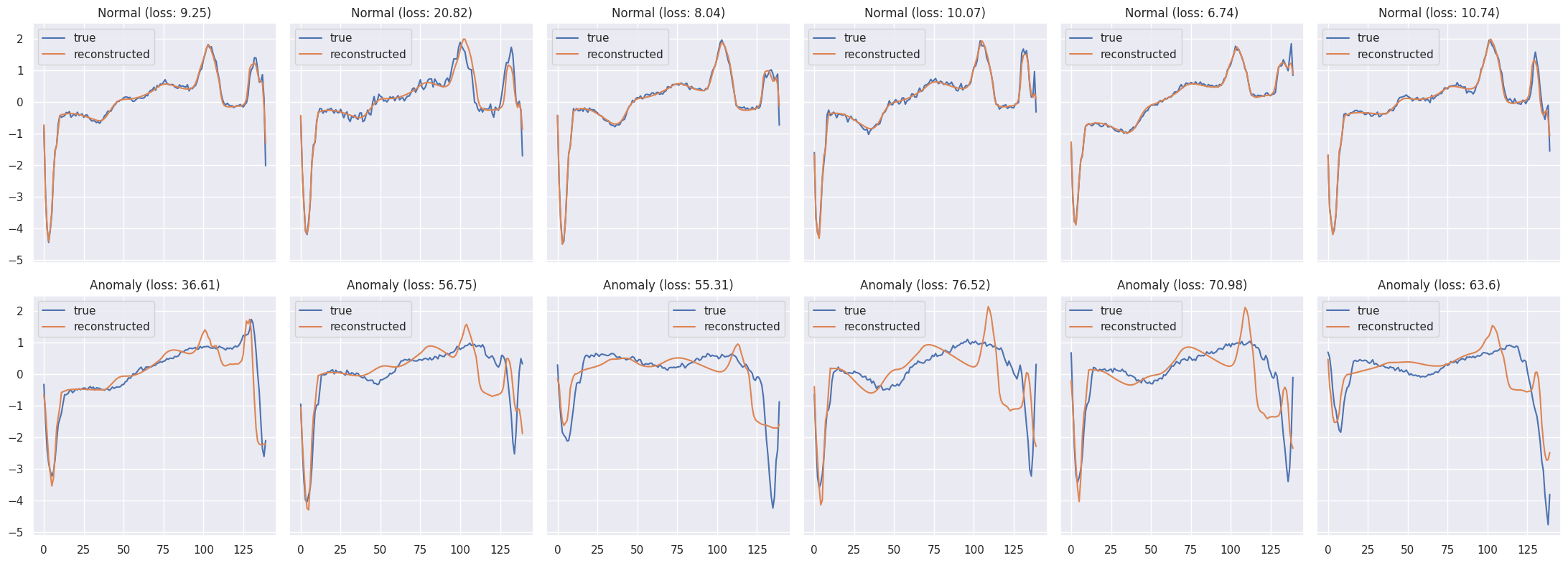
Looking at Examples

We can overlay the real and reconstructed Time Series values to see how close they are. We’ll do it for some normal and anomaly cases:

def plot_prediction(data, model, title, ax):
  predictions, pred_losses = predict(model, [data])

  ax.plot(data, label='true')
  ax.plot(predictions[0], label='reconstructed')
  ax.set_title(f'{title} (loss: {np.around(pred_losses[0], 2)})')
  ax.legend()

fig, axs = plt.subplots(
  nrows=2,
  ncols=6,
  sharey=True,
  sharex=True,
  figsize=(22, 8)
)

for i, data in enumerate(test_normal_dataset[:6]):
  plot_prediction(data, model, title='Normal', ax=axs[0, i])

for i, data in enumerate(test_anomaly_dataset[:6]):
  plot_prediction(data, model, title='Anomaly', ax=axs[1, i])

fig.tight_layout()

Acknowledgments

• Initial version: Mark Neubauer

• Modified from this notebook

© Copyright 2025