Autoencoders#
import os
import subprocess
import random
import numpy as np
import pandas as pd
import matplotlib.pyplot as plt
import seaborn as sns; sns.set_theme()
import warnings; warnings.filterwarnings('ignore')
def wget_data(url: str, local_path='./tmp_data'):
  os.makedirs(local_path, exist_ok=True)

  p = subprocess.Popen(["wget", "-nc", "-P", local_path, url], stderr=subprocess.PIPE, encoding='UTF-8')
  rc = None

  while rc is None:
    line = p.stderr.readline().strip('\n')
    if len(line) > 0:
      print(line)
    rc = p.poll()
Introduction#
 |
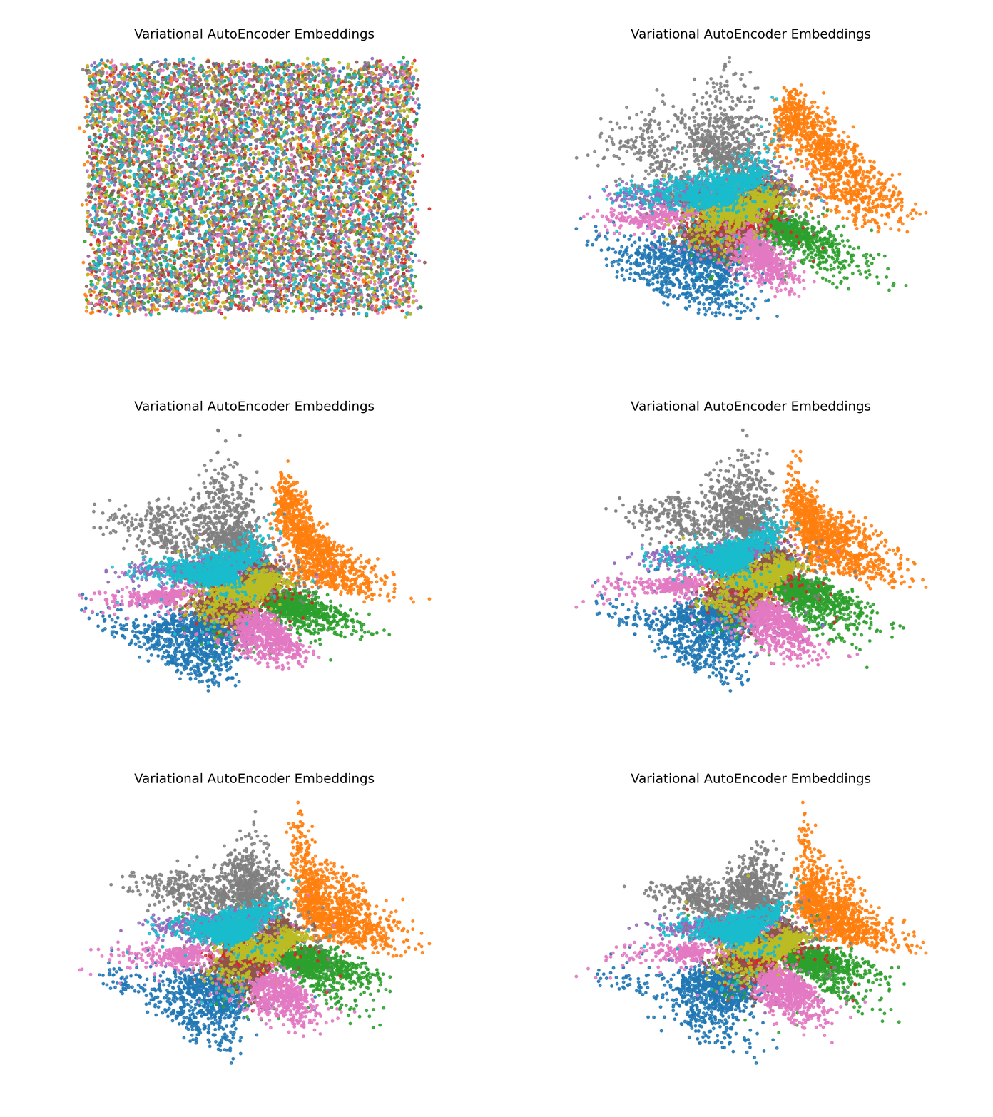 |
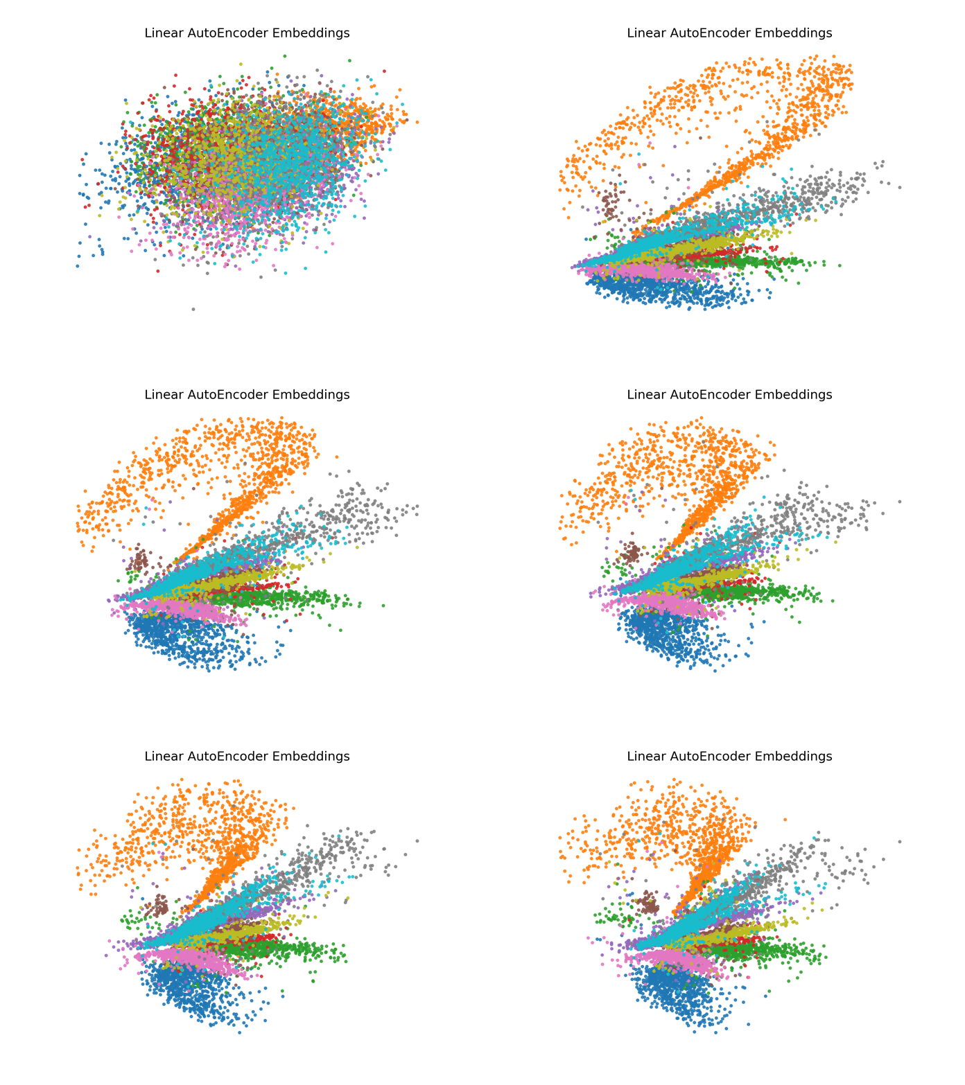
Autoencoders are an incredible compression tool which are used across the board in all types of tasks. Most notable is in many diffusion models such as Stable Diffusion, a Variational AutoEncoder is employed for Latent Space Diffusion modeling (we will see more of this later!). For now though, I want us to get familiar with how AutoEncoders work and build 2 types: (1) Vanilla Autoencoders, and (2) Variational Autoencoders. We will build both a Linear and Convolutional model and the Variational model will be a change from the original Vanilla Autoencoder implementation so you can see what goes into it.
Note: All of our implementations we will do going forward is on MNIST, and that dataset is too simple to give appreciable differences between these architectures! I mainly decided to do this so we can focus on the core ideas of each architecture rather than fiddling around with making the model larger to learn the encodings.
How Does MP4 Compression Work?#
Data Compression is a crucial aspect for Information management. Compression is everywhere! Everyone has seen .mp4 files before, but what does this compression format do?
Instead of storing every frame as an image and storing all the images, MP4 will create reference frames every few frames throughout the video. Then, instead of storing all the pixel values of frames after the reference frame, it will only store what pixels changed from the reference frame.
By doing this, if there is not a lot of movement in the frame, all that redundant data can be thrown out for the compression to occur. Although our filesize has now gone down considerably, when we go to play back the video, the computer needs to perform computations of taking every reference frame and then adding the changes to it to display the future frames. There is a ton more that goes into this (which you can explore), but for now just use this as an analogy for the value of autoenoders.
What is an Autoencoder?#
AutoEncoders are similar to MP4 compression. In data, typically there is a lot of redundant information (correlated features). There are repeating patterns that don’t need to be stored, but instead can be extrapolated from a compressed state.
For example, if I gave you an image with random chunks of it missing, could you fill in the gaps? Of course! And we will take a look at these type of gap-filling architectures in the future, but for now lets explore the basics. More specifically, AutoEncoders fall into the algorithmic category of Unsupervised Dimensionality Reduction.
Below we briefly review the curse of dimensionality and principle components analysis from the Dimensionality notebook since these are used in our analysis and discussion of autoencoders.
Curse of Dimensionality#
We typically describe data by the number of features (or dimensions) it has, but we fall into a problem coined by Richard Bellman, the Curse of Dimensionality. High dimensional data causes a lot of problems:
Lack of interpretability, we cannot visualize more than 3 dimensions at a time!
Sparsity, your data may have a super high dimensionality, but may only occupy small pockets of that vector space.
Complexity, as we increase the number of features, the complexity to train models increase
P > N problem, if you have more features than samples of data, your model may be underdetermined or unsolveable! Genomics has this problem typically, where there may be a few hundred samples and thousands of features.
PCA to the Rescue#
Principal Component Analysis (PCA) attempts to solve exactly this problem.
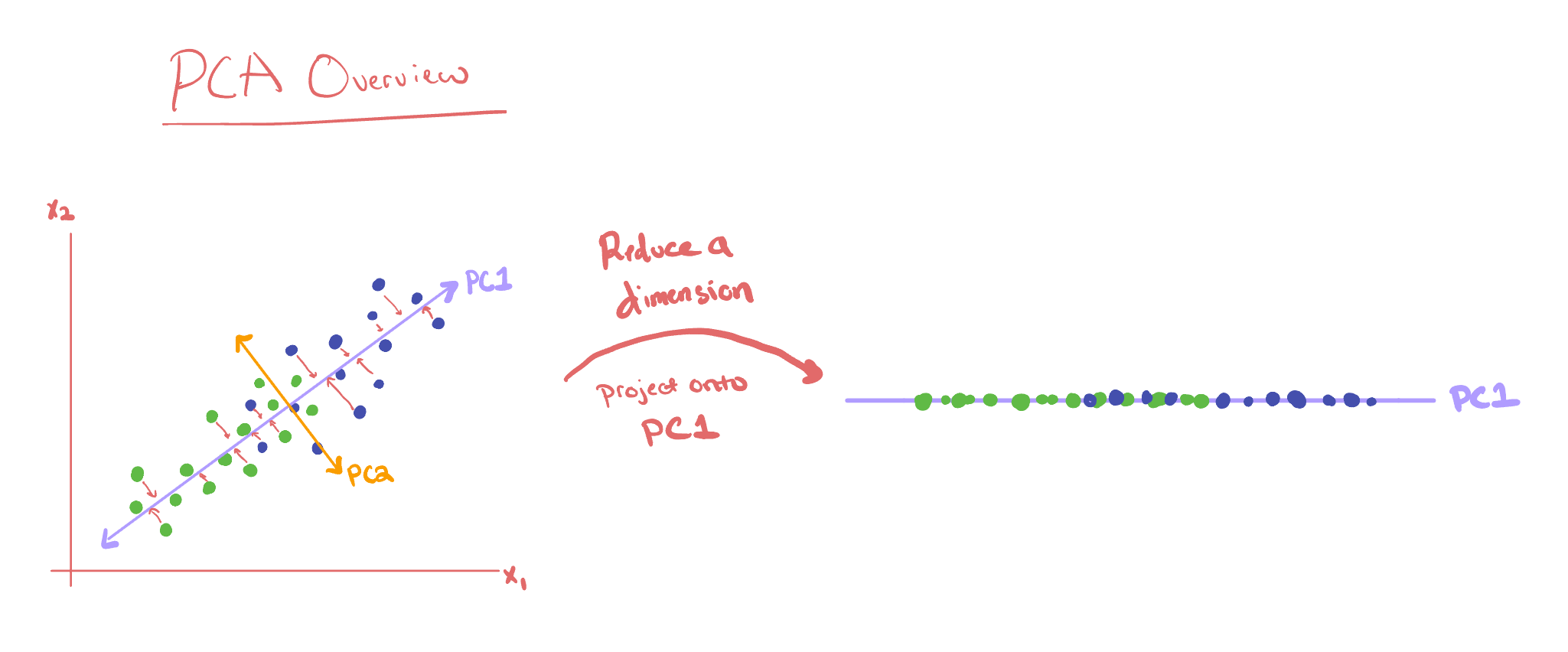
The high-level intuition of PCA is, lets pretend you have dimensions \(x_1, x_2\) and some data that exists in this space. What we want to do is come up with a new set of axis called \(PC_1, PC_2\) (principal component 1 and 2) where each axis represents a direction of highest variance, and all our axis remain orthogonal to each other (just like regular axis).
In the visual above, we have some green and blue dots and we want to train a classifier, but the complexity of two dimensions is too high (just pretend). So we use PCA, which will draw our \(PC_1\), the direction of highest spread (variance) in the dataset and \(PC_2\), the second direction of highest variance that is also orthogonal to the first, and orthogonal axis is centered at the mean of our \(x_1, x_2\) features.
We then throw away \(PC_2\) and project all the data onto \(PC_1\), thus leaving us with only a single dimension (a line). In this line, we can still see a separation between our green and blue dots, therefore a classifier on this one feature will probably be pretty close to training one on the original \(x_1, x_2\) features. If you then have a large number of correlated features in your dataset, you can compress them down into just a few features.
This typically works really well in practice, but there are two limitations to PCA:
The princpal components are linear
Each principal component has to be orthogonal to each other
Data can be complex, messy, and definitely non-linear, so how do Autoencoders address this?
Autoencoders are Non-Linear PCA#
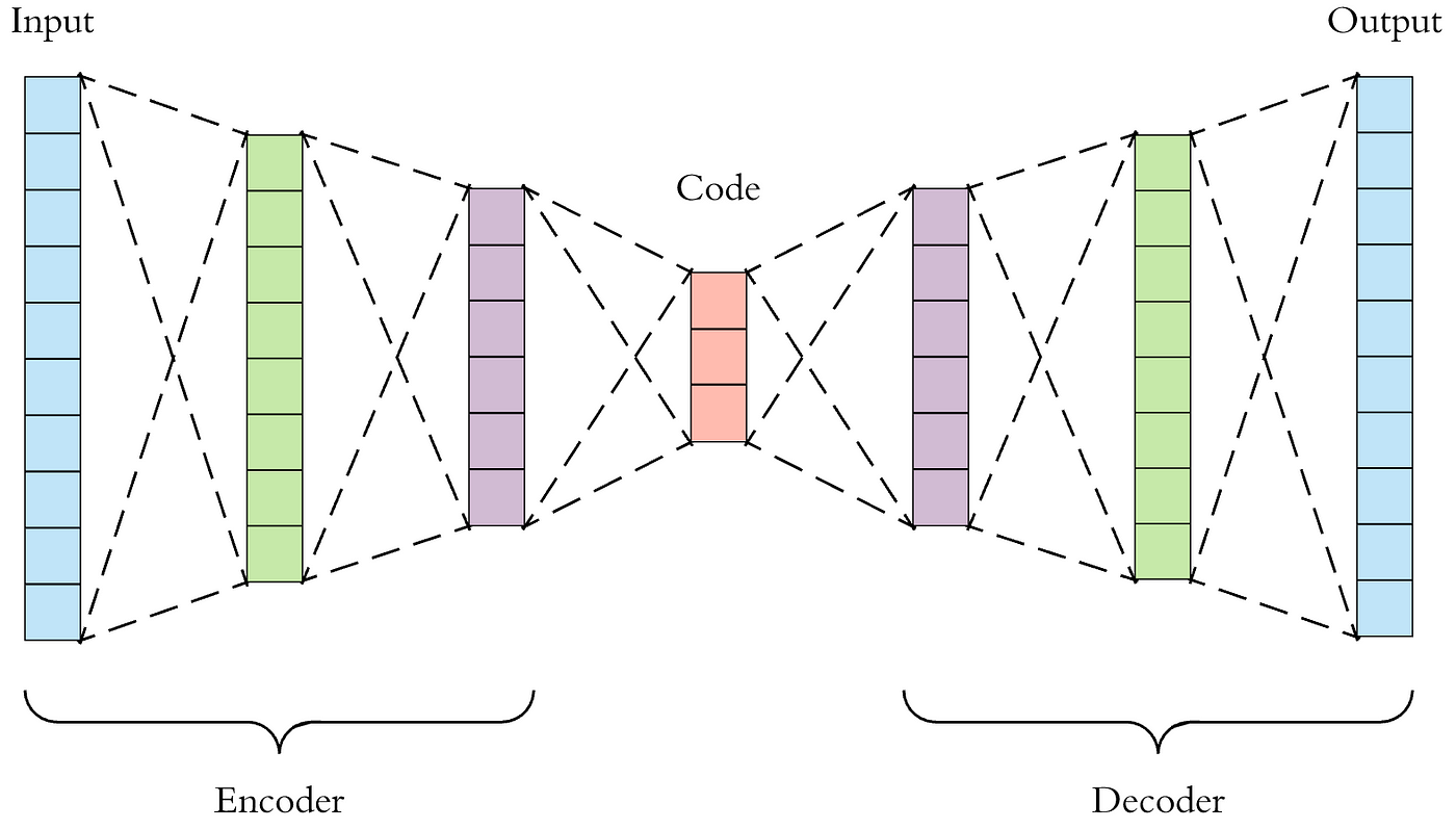
Instead of performing a linear compression via PCA, we can force a Neural Network to compress data (the encoder) and then use the compressed form to recontruct the original data (the decoder). This forces the model to create a low dimensional representation of the input data that is good enough to be used to reconstruct the original data.
The typical form for the autoencoder is this hourglass shape, where the encoder and decoder are mirror images of each other with the most restriction of data flow in the middle (typically called the latent space of the model). It is important for the bottleneck to be sufficiently small, otherwise the model will just learn an identity function. To train this model, all we need to do is pass in data, and then compute a reconstruction loss on the other end to the input.
The architecture you use for the compression and decompression is totally up to you! For images, starting with simple MNIST data for now, we will explore Linear compression and then Convolution compression. What I want to focus on here is how the AutoEncoder learns the latent space. For visualizing the embeddings, we will compress MNIST down to just two numbers so that we go from 28 x 28 = 784 pixels to just two numbers \(\to\) a very high compression factor!
wget_data('https://raw.githubusercontent.com/illinois-mlp/MachineLearningForPhysics/main/data/MNIST/t10k-images-idx3-ubyte', 'tmp_data/MNIST/raw')
wget_data('https://raw.githubusercontent.com/illinois-mlp/MachineLearningForPhysics/main/data/MNIST/t10k-labels-idx1-ubyte',  'tmp_data/MNIST/raw')
wget_data('https://raw.githubusercontent.com/illinois-mlp/MachineLearningForPhysics/main/data/MNIST/train-images-idx3-ubyte', 'tmp_data/MNIST/raw')
wget_data('https://raw.githubusercontent.com/illinois-mlp/MachineLearningForPhysics/main/data/MNIST/train-labels-idx1-ubyte', 'tmp_data/MNIST/raw')
File ‘tmp_data/MNIST/raw/t10k-images-idx3-ubyte’ already there; not retrieving.
File ‘tmp_data/MNIST/raw/t10k-labels-idx1-ubyte’ already there; not retrieving.
File ‘tmp_data/MNIST/raw/train-images-idx3-ubyte’ already there; not retrieving.
File ‘tmp_data/MNIST/raw/train-labels-idx1-ubyte’ already there; not retrieving.
import torch
import torch.nn as nn
import torch.optim as optim
from torch.utils.data import DataLoader
from torchvision import transforms
from torchvision.datasets import MNIST
from tqdm.auto import tqdm
from sklearn.decomposition import PCA

### Stuff to Visualize the Latent Space ###
from celluloid import Camera
from IPython.display import HTML
### Seed Everything ###
torch.manual_seed(0)
torch.cuda.manual_seed(0)
np.random.seed(0)
random.seed(0)

### GENERATE ANIMATIONS ###
generate_anim = False

# I am resizing the 28x28 image to 32x32 just so its a power of 2!
transform = transforms.Compose(
    [
        transforms.Resize((32,32)),
        transforms.ToTensor()
    ]
)

train_set = MNIST('./tmp_data', train=True, transform=transform)
test_set = MNIST('./tmp_data', train=False, transform=transform)

### SET DEVICE ###
device = "cuda" if torch.cuda.is_available() else "cpu"
Basic NonLinear Autoencoder#
Everything about this Nonlinear AutoEncoder is arbritrary. All we care about is to have 28 x 28 outputs going in and 28 x 28 inputs coming out. All the layers are just reasonable guesses for hidden layers, and we included ReLU nonlinearity. Also, the images we are trying to predict have been scaled between 0 and 1, so we want the output of our model to be the same, so that is why we have a sigmoid placed at the end.
class VanillaAutoEncoder(nn.Module):
    def __init__(self, bottleneck_size=2):
        super().__init__()

        self.encoder = nn.Sequential(
            nn.Linear(32*32, 128),
            nn.ReLU(),
            nn.Linear(128, 64),
            nn.ReLU(),
            nn.Linear(64, 32),
            nn.ReLU(),
            nn.Linear(32, bottleneck_size)
        )

        self.decoder = nn.Sequential(
            nn.Linear(bottleneck_size, 32),
            nn.ReLU(),
            nn.Linear(32, 64),
            nn.ReLU(),
            nn.Linear(64, 128),
            nn.ReLU(),
            nn.Linear(128, 32*32),
            nn.Sigmoid()
        )

    def forward_enc(self, x):
        return self.encoder(x)

    def forward_dec(self, x):
        x = self.decoder(x)
        x = x.reshape(-1,1,32,32)
        return x

    def forward(self, x):

        batch, channels, height, width = x.shape

        ### Flatten Image to Vector ###
        x = x.flatten(1)

        ### Pass Through Encoder ###
        enc = self.forward_enc(x)

        ### Pass Through Decoder ###
        dec = self.forward_dec(enc)

        return enc, dec
Super Simple Training Script#
There isn’t anything fancy going on in this training script. We just pass in is the model we want to train, the datasets, the batch size we want to use, as well as the number of training iterations and how often we want to evaluate the model with the testing data. The only extra thing added in is when we evaluate the model, we will store all the encoded images so we can plot the encodings over the duration of the training later.
def train(model,
          train_set,
          test_set,
          batch_size,
          training_iterations,
          evaluation_iterations,
          verbose=False):

    print("Training Model!")
    print(model)

    ### Set the Device ###
    device = "cuda" if torch.cuda.is_available() else "cpu"

    ### Define the Model and Place on Device ###
    model = model.to(device)

    ### Set the Dataloaders ###
    trainloader = DataLoader(train_set, batch_size=batch_size, shuffle=True, num_workers=8)
    testloader = DataLoader(test_set, batch_size=batch_size, shuffle=False, num_workers=8)

    ### Set the Optimizer ###
    optimizer = optim.Adam(model.parameters(), lr=0.0005)

    ### Some List for logging ###
    train_loss = []
    evaluation_loss = []
    train_losses = []
    evaluation_losses = []

    ### List to store Encoded Data when Evaluating ###
    encoded_data_per_eval = []

    ### Create a Progress Bar ###
    pbar = tqdm(range(training_iterations))

    train = True
    step_counter = 0
    while train:

        for images, labels in trainloader:

            images = images.to(device)
            encoded, reconstruction = model(images)

            ### Simple MSE Loss ###
            loss = torch.mean((images - reconstruction)**2)
            train_loss.append(loss.item())

            loss.backward()
            optimizer.step()
            optimizer.zero_grad()

            if step_counter % evaluation_iterations == 0:

                model.eval()
                encoded_evaluations = []

                for images, labels in testloader:

                    images = images.to(device)
                    encoded, reconstruction = model(images)
                    loss = torch.mean((images - reconstruction)**2)
                    evaluation_loss.append(loss.item())

                    ### Store the Encoded Image with their Labels ###
                    encoded, labels = encoded.cpu().flatten(1), labels.reshape(-1,1)
                    encoded_evaluations.append(torch.cat((encoded, labels), axis=-1))

                ### Store All Testing Encoded Images ###
                encoded_data_per_eval.append(torch.concatenate(encoded_evaluations).detach())

                train_loss = np.mean(train_loss)
                evaluation_loss = np.mean(evaluation_loss)

                train_losses.append(train_loss)
                evaluation_losses.append(evaluation_loss)

                if verbose:
                    print("Training Loss", train_loss)
                    print("Evaluation Loss", evaluation_loss)

                ### Reset For Next Evaluation ###
                train_loss = []
                evaluation_loss = []

                model.train()

            step_counter += 1
            pbar.update(1)

            if step_counter >= training_iterations:
                print("Completed Training!")
                train = False
                break

    ### Store All Encoded Data as Numpy Arrays for each Eval Iteration ###
    encoded_data_per_eval = [np.array(i) for i in encoded_data_per_eval]

    print("Final Training Loss", train_losses[-1])
    print("Final Evaluation Loss", evaluation_losses[-1])

    return model, train_losses, evaluation_losses, encoded_data_per_eval

vanilla_model = VanillaAutoEncoder(bottleneck_size=2)
vanilla_model, train_losses, evaluation_losses, vanilla_encoded_data = train(vanilla_model,
                                                                             train_set,
                                                                             test_set,
                                                                             batch_size=64,
                                                                             training_iterations=25000,
                                                                             evaluation_iterations=250)
Training Model!
VanillaAutoEncoder(
  (encoder): Sequential(
    (0): Linear(in_features=1024, out_features=128, bias=True)
    (1): ReLU()
    (2): Linear(in_features=128, out_features=64, bias=True)
    (3): ReLU()
    (4): Linear(in_features=64, out_features=32, bias=True)
    (5): ReLU()
    (6): Linear(in_features=32, out_features=2, bias=True)
  )
  (decoder): Sequential(
    (0): Linear(in_features=2, out_features=32, bias=True)
    (1): ReLU()
    (2): Linear(in_features=32, out_features=64, bias=True)
    (3): ReLU()
    (4): Linear(in_features=64, out_features=128, bias=True)
    (5): ReLU()
    (6): Linear(in_features=128, out_features=1024, bias=True)
    (7): Sigmoid()
  )
)
Completed Training!
Final Training Loss 0.028624614074826242
Final Evaluation Loss 0.029113601596587022
Plotting the Embedded Space through Training#
We can now write a function that takes in encoded_data_per_eval from our output of the training, and then create an animation of the embeddings space to see how the Neural Network Learns.
def build_embedding_animation(encoded_data_per_eval, iterations_per_eval=100):

    fig, ax = plt.subplots()

    camera = Camera(fig)

    for idx, encoding in enumerate(encoded_data_per_eval):

        encoding = pd.DataFrame(encoding, columns=["x", "y", "class"])
        encoding = encoding.sort_values(by="class")
        encoding["class"] = encoding["class"].astype(int).astype(str)

        for grouper, group in encoding.groupby("class"):
            plt.scatter(x=group["x"], y=group["y"], label=grouper, alpha=0.8, s=5)

        ax.text(0.4, 1.01, f"Step {idx*iterations_per_eval}", transform=ax.transAxes, fontsize=12)
        ax.set_xlabel("x")
        ax.set_ylabel("y")

        camera.snap()

    plt.close()
    anim = camera.animate(blit=True)

    return anim

def build_embedding_plot(encoding, title):
    encoding = pd.DataFrame(encoding, columns=["x", "y", "class"])
    encoding = encoding.sort_values(by="class")
    encoding["class"] = encoding["class"].astype(int).astype(str)

    for grouper, group in encoding.groupby("class"):
        plt.scatter(x=group["x"], y=group["y"], label=grouper, alpha=0.8, s=5)

    plt.title(title)
    plt.xlabel("x")
    plt.ylabel("y")
    plt.show()

if generate_anim:
    anim = build_embedding_visual(vanilla_encoded_data)
    HTML(anim.to_jshtml())

else:
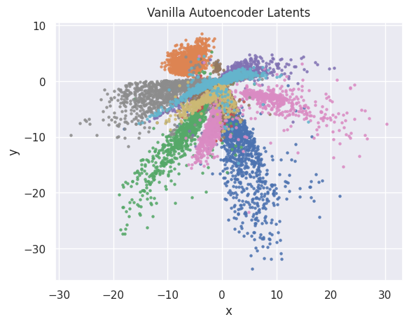
    build_embedding_plot(vanilla_encoded_data[-1], "Vanilla Autoencoder Latents")
Just for Fun: A Linear Autoencoder!#
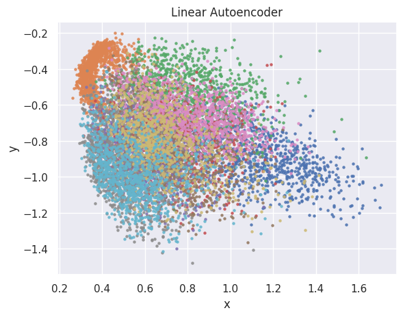
Although this isn’t exactly PCA because we have no orthogonality restrictions on the components, we expect that a linear autoencoder would produce somewhat similar output to what PCA produces.
class LinearAutoEncoder(nn.Module):
    def __init__(self, bottleneck_size=2):
        super().__init__()

        self.encoder = nn.Sequential(
            nn.Linear(32*32, bottleneck_size),
        )

        self.decoder = nn.Sequential(
            nn.Linear(bottleneck_size, 32*32),
        )

    def forward(self, x):

        batch, channels, height, width = x.shape

        ### Flatten Image to Vector ###
        x = x.flatten(1)

        ### Pass Through Encoder ###
        enc = self.encoder(x)

        ### Pass Through Decoder ###
        dec = self.decoder(enc)

        ### Put Decoded Image Back to Original Shape ###
        dec = dec.reshape(batch, channels, height, width)

        return enc, dec
linear_model = LinearAutoEncoder(bottleneck_size=2)
model, train_losses, evaluation_losses, linear_encoded_data = train(linear_model,
                                                                    train_set,
                                                                    test_set,
                                                                    batch_size=64,
                                                                    training_iterations=25000,
                                                                    evaluation_iterations=250)
if generate_anim:
    anim = build_embedding_visual(linear_encoded_data)
    HTML(anim.to_jshtml())

else:
    build_embedding_plot(linear_encoded_data[-1], "Linear Autoencoder")
Training Model!
LinearAutoEncoder(
  (encoder): Sequential(
    (0): Linear(in_features=1024, out_features=2, bias=True)
  )
  (decoder): Sequential(
    (0): Linear(in_features=2, out_features=1024, bias=True)
  )
)
Completed Training!
Final Training Loss 0.04622595304250717
Final Evaluation Loss 0.04618092600232477
Comparisons to PCA#
data = np.array(torch.cat([d[0].flatten(1) for d in test_set], dim=0))
labels = np.array([d[1] for d in test_set]).reshape(-1,1)

### PCA Encodings ###
pca = PCA(n_components=2)
pca_encoding = pca.fit_transform(data)
pca_encoding = np.concatenate((pca_encoding, labels), axis=-1)
pca_encoding = pd.DataFrame(pca_encoding, columns=["x", "y", "class"])
pca_encoding = pca_encoding.sort_values(by="class")
pca_encoding["class"] = pca_encoding["class"].astype(int).astype(str)

### Grab Last Linear Encodings ###
linauto_encoding = linear_encoded_data[-1]
linauto_encoding = pd.DataFrame(linauto_encoding, columns=["x", "y", "class"])
linauto_encoding = linauto_encoding.sort_values(by="class")
linauto_encoding["class"] = linauto_encoding["class"].astype(int).astype(str)

### Lets Plot it All Now! ###
f, (ax1,ax2) = plt.subplots(1,2, figsize=(15,5))

### Plot PCA Plot ###
for grouper, group in pca_encoding.groupby("class"):
    ax1.scatter(x=group["x"], y=group["y"], label=grouper, alpha=0.8, s=5)
ax1.legend()
ax1.set_xlabel("x")
ax1.set_ylabel("y")
ax1.set_title("PCA Embeddings")

for grouper, group in linauto_encoding.groupby("class"):
    ax2.scatter(x=group["x"], y=group["y"], label=grouper, alpha=0.8, s=5)
ax2.legend()
ax2.set_xlabel("x")
ax2.set_ylabel("y")
ax2.set_title("Linear AutoEncoder Embeddings")

plt.show()
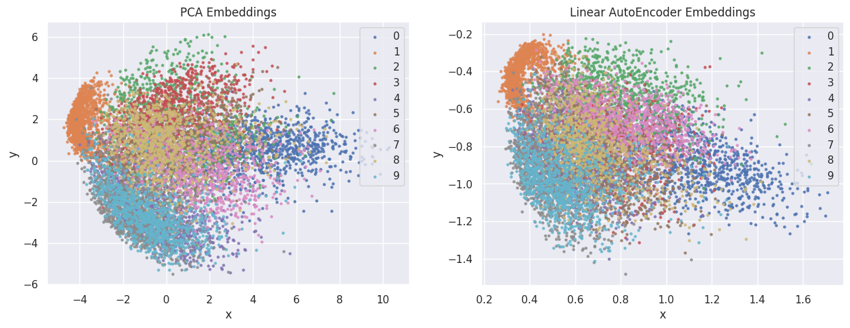
These actually look pretty similar! Disregarding the scale, the Linear Autoencoder is a seems like a rotated version of the PCA embeddings. (The Linear AutoEncoder can also change every time you run it just due to randomness of training). If they look similar, then what do the weight vectors of each principal component look like? Are they orthogonal?
### Principal Component Vectors ###
pc_1, pc_2 = torch.tensor(pca.components_[0]), torch.tensor(pca.components_[1])
print("Angle Between PCA Principal Components", torch.rad2deg(torch.acos(torch.dot(pc_1, pc_2))).item())

### Linear AutoEncoder Projection Vectors ###
model_weights = model.encoder[0].weight

weight_vector_1, weight_vector_2 = model_weights[0].cpu(), model_weights[1].cpu()
weight_vector_1 = weight_vector_1 / torch.norm(weight_vector_1)
weight_vector_2 = weight_vector_2 / torch.norm(weight_vector_2)

print("Angle Between AutoEncoder Vectors", torch.rad2deg(torch.acos(torch.dot(weight_vector_1, weight_vector_2))).item())
Angle Between PCA Principal Components 90.0
Angle Between AutoEncoder Vectors 87.34716796875
It looks like the best projection vectors the model could create were almost Orthogonal! This shows that AutoEncoders can closely approximate PCA by using Gradient Descent rather than expensive eigenvalue decompositions on large datasets.
Example: Spectra Data#
Re-use the spectral data for an example.
wget_data('https://raw.githubusercontent.com/illinois-mlp/MachineLearningForPhysics/main/data/spectra_data.hf5')
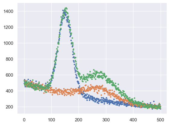
Recall that there are only 200 samples in 500 dimensions:
for i in (0, 6, 7):
    plt.plot(X[i], '.', ms=5)
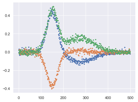
Pytorch layers initializes parameters assuming that inputs are roughly normalized:
X0 = np.mean(X, axis=0)
Xmax = np.max(np.abs(X - X0))
Xn = (X - X0) / Xmax
original = lambda x: Xmax * x + X0
assert np.allclose(X, original(Xn))
for i in (0, 6, 7):
    plt.plot(Xn[i], '.', ms=5)
Build simple Pytorch autoencoder model:
Train the model
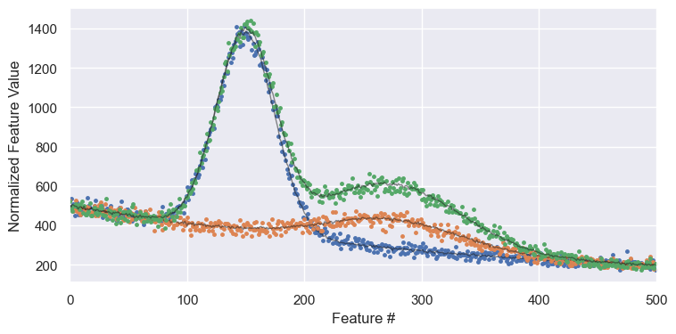
def plot_reconstructed(Xn, model):
    predictions = model.predict(
        input_fn=tf.estimator.inputs.numpy_input_fn(
            x={'X': Xn}, y=None, num_epochs=1, shuffle=False))
    N, D = Xn.shapec
    fig = plt.figure(figsize=(8.5, 4))
    for i, pred in enumerate(predictions):
        Xr = original(pred['output'])
        plt.plot(original(Xn[i]), '.', ms=5)
        plt.plot(Xr, 'k-', lw=1, alpha=0.5)
    plt.xlim(-0.5, D+0.5)
    plt.xlabel('Feature #')
    plt.ylabel('Normalized Feature Value')

plot_reconstructed(Xn[[0, 6, 7]], model=autoenc)
WARNING:tensorflow:From /usr/local/lib/python3.11/site-packages/tensorflow/python/saved_model/model_utils/export_utils.py:366: PredictOutput.__init__ (from tensorflow.python.saved_model.model_utils.export_output) is deprecated and will be removed in a future version.
Instructions for updating:
Use tf.keras instead.
Convolutional Autoencoder#
There are two ways you can do Convolutional Autoencoders. The first way is have some convolutional compression (decrease image size, increase channels), then flatten with a few linear layers down to the bottleneck size you want, and then have some decoder linear layers followed by some Transpose Convolutions to upsample back to the image shape.
The second is to forgo the linear layers and only have convolutions compression and transpose convolutional decompression. We will be doing the second method as this type of architecture will repeat again in the future. Remember, Convolutions work in the channel space and we never will compress down to linear (pixel) space.
Again, there is absolutely no reason for any of the architecture decisions I made, i just picked stuff randomly so it worked. But, there is one thing to talk about and that is compression ratio!
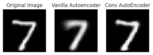
In our Vanilla Autoencoder we used 2 numbers to represent all 1024 pixels (there are 1024 pixels instead of 784 bceause we resized MNIST to 32x32). In this example, you will see our AutoEncoder will compress images down to a 4 Channels x 4 Height x 4 Width, so effectively 64 numbers, giving the model a lot more room to express the images. So although our compression ratio is not as high, we should see better reconstructions at least.
class ConvolutionalAutoEncoder(nn.Module):
    def __init__(self, in_channels=1, channels_bottleneck=4):
        super().__init__()

        self.bottleneck = channels_bottleneck
        self.in_channels = in_channels

        self.encoder_conv = nn.Sequential(

            ### Convolutional Encoding ###
            nn.Conv2d(in_channels=in_channels, out_channels=8, kernel_size=5, stride=2, padding=1, bias=False),
            nn.BatchNorm2d(8),
            nn.ReLU(),

            nn.Conv2d(in_channels=8, out_channels=16, kernel_size=3, stride=2, padding=1, bias=False),
            nn.BatchNorm2d(16),
            nn.ReLU(),

            nn.Conv2d(in_channels=16, out_channels=self.bottleneck, kernel_size=3, stride=2, padding=1, bias=False),
            nn.BatchNorm2d(self.bottleneck),
            nn.ReLU()
        )

        self.decoder_conv = nn.Sequential(
            nn.ConvTranspose2d(in_channels=self.bottleneck, out_channels=16, kernel_size=3, stride=2, bias=False),
            nn.BatchNorm2d(16),
            nn.ReLU(),

            nn.ConvTranspose2d(in_channels=16, out_channels=8, kernel_size=3, stride=2, padding=1, bias=False),
            nn.BatchNorm2d(8),
            nn.ReLU(),

            nn.ConvTranspose2d(in_channels=8, out_channels=in_channels, kernel_size=2, stride=2, padding=1),
            nn.Sigmoid()
        )

    def forward_enc(self, x):
        batch_size, num_channels, height, width = x.shape
        conv_enc = self.encoder_conv(x)
        return conv_enc

    def forward_dec(self, x):
        batch_size = x.shape[0]
        x = x.reshape((batch_size, self.bottleneck, 4, 4))
        conv_dec = self.decoder_conv(x)
        return conv_dec

    def forward(self, x):
        batch_size, num_channels, height, width = x.shape
        enc = self.forward_enc(x)
        dec = self.forward_dec(enc)
        return enc, dec

conv_model = ConvolutionalAutoEncoder()
conv_model, train_losses, evaluation_losses, conv_encoded_data_per_eval = train(conv_model,
                                                                                train_set,
                                                                                test_set,
                                                                                batch_size=64,
                                                                                training_iterations=25000,
                                                                                evaluation_iterations=250)
Training Model!
ConvolutionalAutoEncoder(
  (encoder_conv): Sequential(
    (0): Conv2d(1, 8, kernel_size=(5, 5), stride=(2, 2), padding=(1, 1), bias=False)
    (1): BatchNorm2d(8, eps=1e-05, momentum=0.1, affine=True, track_running_stats=True)
    (2): ReLU()
    (3): Conv2d(8, 16, kernel_size=(3, 3), stride=(2, 2), padding=(1, 1), bias=False)
    (4): BatchNorm2d(16, eps=1e-05, momentum=0.1, affine=True, track_running_stats=True)
    (5): ReLU()
    (6): Conv2d(16, 4, kernel_size=(3, 3), stride=(2, 2), padding=(1, 1), bias=False)
    (7): BatchNorm2d(4, eps=1e-05, momentum=0.1, affine=True, track_running_stats=True)
    (8): ReLU()
  )
  (decoder_conv): Sequential(
    (0): ConvTranspose2d(4, 16, kernel_size=(3, 3), stride=(2, 2), bias=False)
    (1): BatchNorm2d(16, eps=1e-05, momentum=0.1, affine=True, track_running_stats=True)
    (2): ReLU()
    (3): ConvTranspose2d(16, 8, kernel_size=(3, 3), stride=(2, 2), padding=(1, 1), bias=False)
    (4): BatchNorm2d(8, eps=1e-05, momentum=0.1, affine=True, track_running_stats=True)
    (5): ReLU()
    (6): ConvTranspose2d(8, 1, kernel_size=(2, 2), stride=(2, 2), padding=(1, 1))
    (7): Sigmoid()
  )
)
Completed Training!
Final Training Loss 0.004364030033349991
Final Evaluation Loss 0.004125288044025374
generated_index = 0
image, label = test_set[generated_index]

_, vanilla_reconstructed = vanilla_model(image.unsqueeze(0).to(device))
_, conv_reconstructed = conv_model(image.unsqueeze(0).to(device))

vanilla_reconstructed = vanilla_reconstructed.to("cpu").detach().numpy()
conv_reconstructed = conv_reconstructed.to("cpu").detach().numpy()

fig, ax = plt.subplots(1,3)

ax[0].imshow(image.squeeze(), cmap="gray")
ax[0].set_title("Original Image")
ax[0].set_xticklabels([])
ax[0].set_yticklabels([])
ax[0].axis("off")

ax[1].imshow(vanilla_reconstructed.squeeze(), cmap="gray")
ax[1].set_title("Vanilla Autoencoder")
ax[1].set_xticklabels([])
ax[1].set_yticklabels([])
ax[1].axis("off")

ax[2].imshow(conv_reconstructed.squeeze(), cmap="gray")
ax[2].set_title("Conv AutoEncoder")
ax[2].set_xticklabels([])
ax[2].set_yticklabels([])
ax[2].axis("off")

plt.show()
What about Generating New Images?!?#
Until now we have only been looking at our Encoder, which takes an image and compresses it down. What about our Decoder? Lets take our Vanilla Autoencoder for example. If we gave it our own two numbers, will it generate any images?
Of course! Lets try this exercise, we have our encoded testing data, lets find the median 2 number encodings for each digit and pass them through our decoder to see what it makes!
final_embeddings = vanilla_encoded_data[-1]

avg_digit_embeddings = []

for i in range(10):
    avg_embeddings = np.median(final_embeddings[final_embeddings[:, 2] == i][:, :2], axis=0)
    avg_digit_embeddings.append(avg_embeddings)

avg_digit_embeddings = torch.tensor(np.array(avg_digit_embeddings))
pred_images = vanilla_model.forward_dec(avg_digit_embeddings.to(device))

fig, axes = plt.subplots(1,10, figsize=(15,5))
for idx, img in enumerate(pred_images):
    img = img.squeeze().detach().cpu().numpy()
    axes[idx].imshow(img, cmap="gray")
    axes[idx].set_xticklabels([])
    axes[idx].set_yticklabels([])
    axes[idx].axis("off")

fig.subplots_adjust(wspace=0, hspace=0)

plt.show()

Interpolating the Space#
So our generations using the Vanilla Autoencoder are alright, not the best but maybe model tuning would improve it. But the bigger question is, why don’t we use AutoEncoders more for generation? You give it some numbers and it can create what you want! The problem is that the generation space is not compact. Here is again the embedded space from the Vanilla Autoencoder:
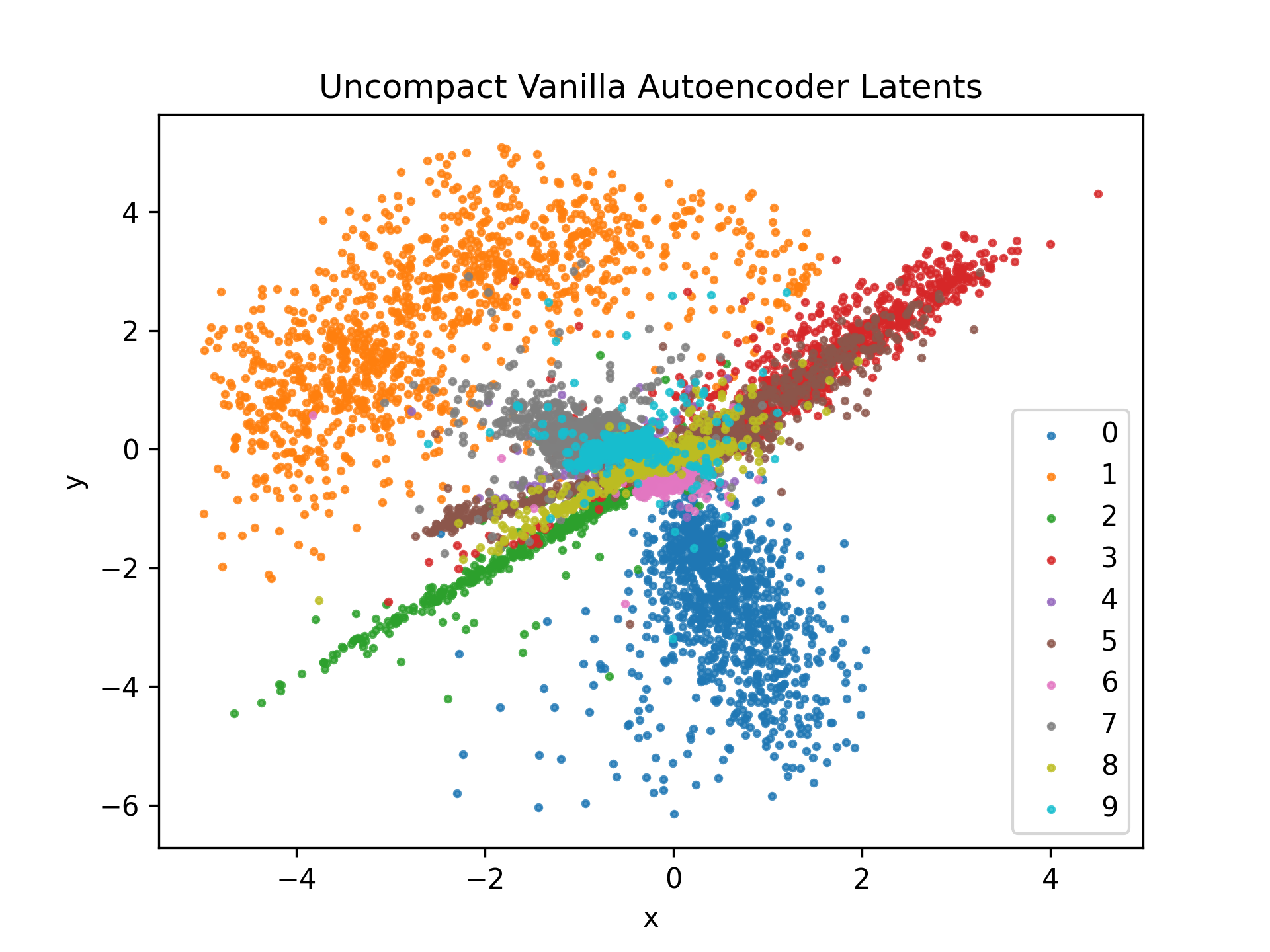
Note: might look a bit different from the actual Embeddings above, I just saved this during a one of the training runs
Notice how the class are totally broken with large amounts of whitespace in between. Many of them also look like they have been stretched out into strands of vector space from the center.
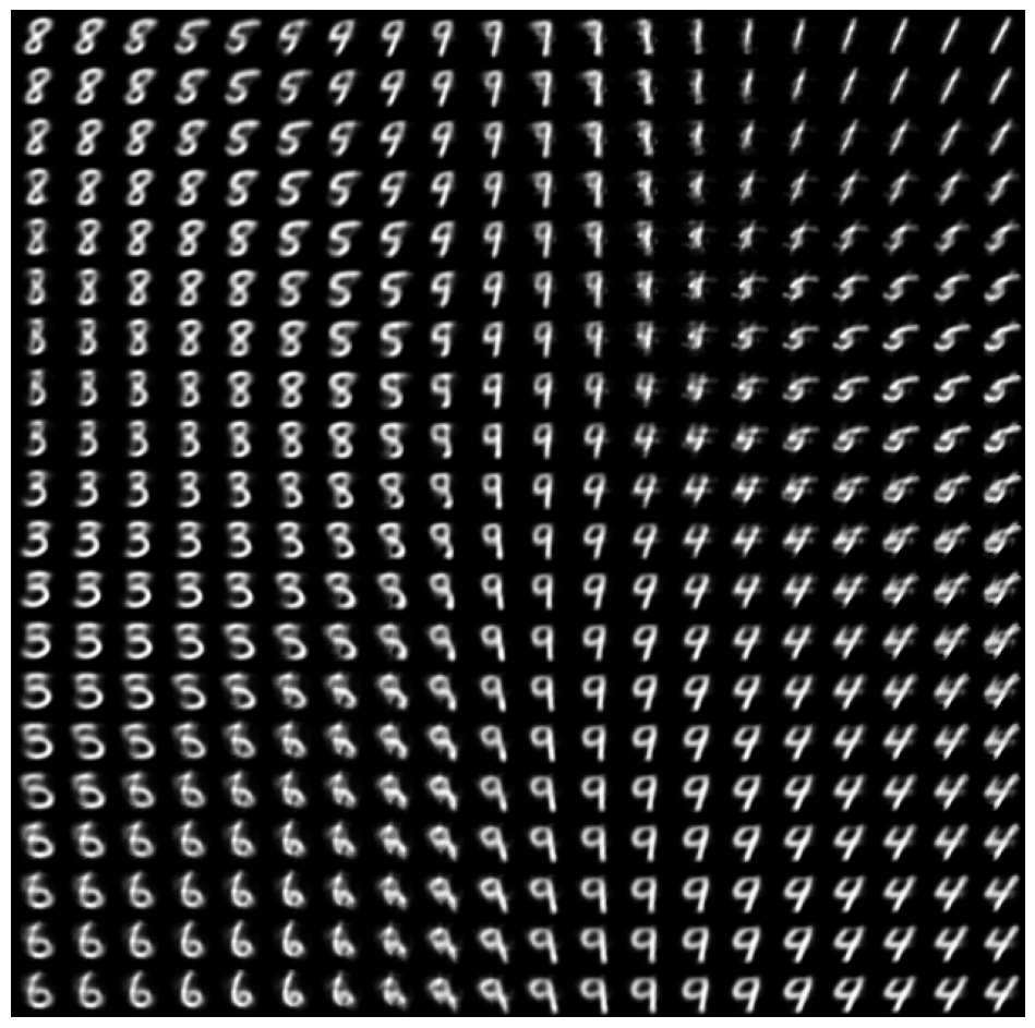
Lets try to interpolate the vector space then. What this means is that we will create a grid of values over a range of \(X\) and \(Y\) values and then plot what the image generated from a point taken from that space looks like. If we sample points from where the actual encodings are, we should have pretty good results, but if we sample from where there is whitespace between the encodings, the generations will be pretty bad.
def interpolate_space(model, x_range=(-3,3), y_range=(-3,3), num_steps=20):

    device = "cuda" if torch.cuda.is_available() else "cpu"
    model = model.to(device)

    x_space = np.linspace(x_range[0], x_range[1], num_steps)
    y_space = np.linspace(y_range[0], y_range[1], num_steps)

    points = []
    for x in x_space:
        for y in y_space:
            points.append([x,y])

    points = torch.tensor(points, dtype=torch.float32).to(device)

    ### Pass Through Model Decoder and Reshape ###
    dec = model.forward_dec(points).detach().cpu()
    dec = dec.reshape((num_steps,num_steps, *dec.shape[1:]))

    fig, ax = plt.subplots(num_steps,num_steps, figsize=(12,12))

    for x in range(num_steps):
        for y in range(num_steps):
            img = np.array(dec[x,y].permute(1,2,0))
            ax[x,y].imshow(img, cmap="gray")
            ax[x,y].set_xticklabels([])
            ax[x,y].set_yticklabels([])
            ax[x,y].axis("off")

    fig.subplots_adjust(wspace=0, hspace=0)

interpolate_space(vanilla_model)
Moving on to Variational Autoencoders#
This is Super Important: Why can’t we generate anything from our Convolutional AutoEncoder?
This is because our convolutional autoencoder compresses our data down to 64 numbers (as a 4 x 4 x 4 cube). I have no idea what the vector space for that 64 values looks like. We dont know where the numbers are, or where we can get good generations. We could probe the model and find them but this isnt practical as the model becomes more complex, and it will be hard to find consistent generations. But what if instead of mapping to some arbritrary latent space like we are doing, if we mapped to a specific one with a known distribution?
This is exactly what Variational AutoEncoders do!
Not only do they need to perform the reconstruction loss like we have already, but the latent distribution is forced to follow some known probability distribution (typically a Normal distribution). If we know the latent space is a Standard Normal distribution, it is very easy to sample from, because we know exactly where the bulk of the data is! In the case of our Convolutional model, we could just pass in gaussian noise to our decoder (in the shape 4 x 4 x 4) and generate away!
Acknowledgments#
Initial version: Mark Neubauer
Modified from the following tutorial
© Copyright 2026
