Attention#
Since its introduction via the original transformer paper (Attention Is All You Need), self-attention has become a cornerstone of many state-of-the-art deep learning models, particularly in the field of Natural Language Processing (NLP). Since self-attention is now everywhere, it’s important to understand how it works. This lecture provides and overview of the key aspects of the attention mechanism and details (code) on how it works.
Although attention was mainly intended for use in sequence modeling, it has found its way into Computer Vision, Graphs and basically every domain, demonstrating the flexibility of the architecture. We will discuss attention from a sequence modeling perspective just to build intuition on how this works.
Recap: Recurrent Neural Networks#
To start the explanation, lets reference back the original sequence modeling mechanism: Recurrent Neural Networks (RNNs). You might review the RNN part of this notebook from earlier in the course.
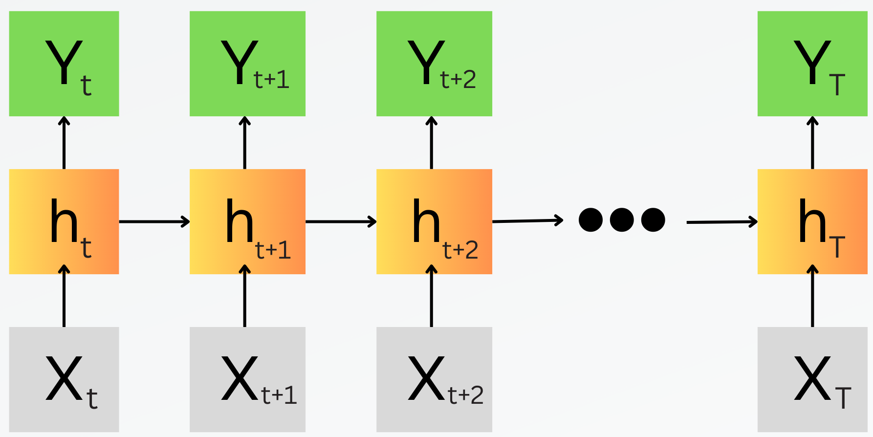
In recurrent neural networks, what we typically do is take our sequence and pass in a single timestep at a time and produce an output. This means when we pass in \(x_1\) we create a hidden state \(h_1\) that captures all the relevant information in the input, and this hidden state then is used to produce the output \(y_1\). Now what makes it an RNN is when we pass in the second timestep \(x_2\) to produce the hidden state \(h_2\), the hidden state already contains information about the past \(h_1\) Therefore our output of \(y_2\) is informed both by information from \(x_2\) and \(x_1\) encoded through the hidden states. If we keep this going, when we want to make a prediction at \(y_{100}\), we will be using a hidden state that has encoded information of all the inputs \(x_1\) to \(x_{100}\).
Everything explained so far is a causal RNN which makes a prediction of some timestep \(t\) by using all of the input timesteps \(<=t\). We can easily expand this to make a bidirectional RNN to make a prediction at time \(t\) by looking at the entire sequence as well. In this case we will really have two hidden states - one that looks backwards and another that looks forward.
Whether you use causal or bidirectional depends a lot on what you want to do. If you want to do Name Entity Recognition (i.e. determine if each word in a sentence is an entity), you can look at the entire sentence to do this. On the other hand if you want to forecast the future, like a stock price, then you have to use causal as you can only look at the past to predict the future.
All this sounds well and good, but there was one glaring problem: Memory. The hidden states we use to encode the history can only contain so much information, i.e. as the sequence length becomes longer the model will have to start to forget based on memory limitations. This matters a lot for things like MLP, as there may be imporant relations between parts of a book that are pages, or even chapters, apart. To solve this issue, Attention Augmented RNNs were introduced in the paper Neural Machine Translation By Jointly Learning To Align and Translate.
Attention Augmented RNN#
If I had to use two words to define attention it would be: Weighted Average. In Attention Augmented RNN paper, the authors call the hidden states annotations, but they are the same thing as attention.
So lets go back to our RNN again. Before we do our prediction for \(y_t\), we have a sequence of hidden states \(h_t\) that contain the information about the sequence \(x_t\) itself produced from the RNN mechanism. Again, the problem is that \(h_t\) for large values of \(t\) will have forgotten imporant information about early \(x_t\) values with small values of \(t\). So what if we got everyone to know each other again? We can produce a context vector \(c_i\) that is a weighted average of all the hidden states in the case of a bidirectional architecture, or just the previous hidden states in a causal architecture. This means at any time of the context vector \(c_t\), it will be a weighted average of all of the timesteps so it is reminded about more distant timesteps, solving our memory problem!
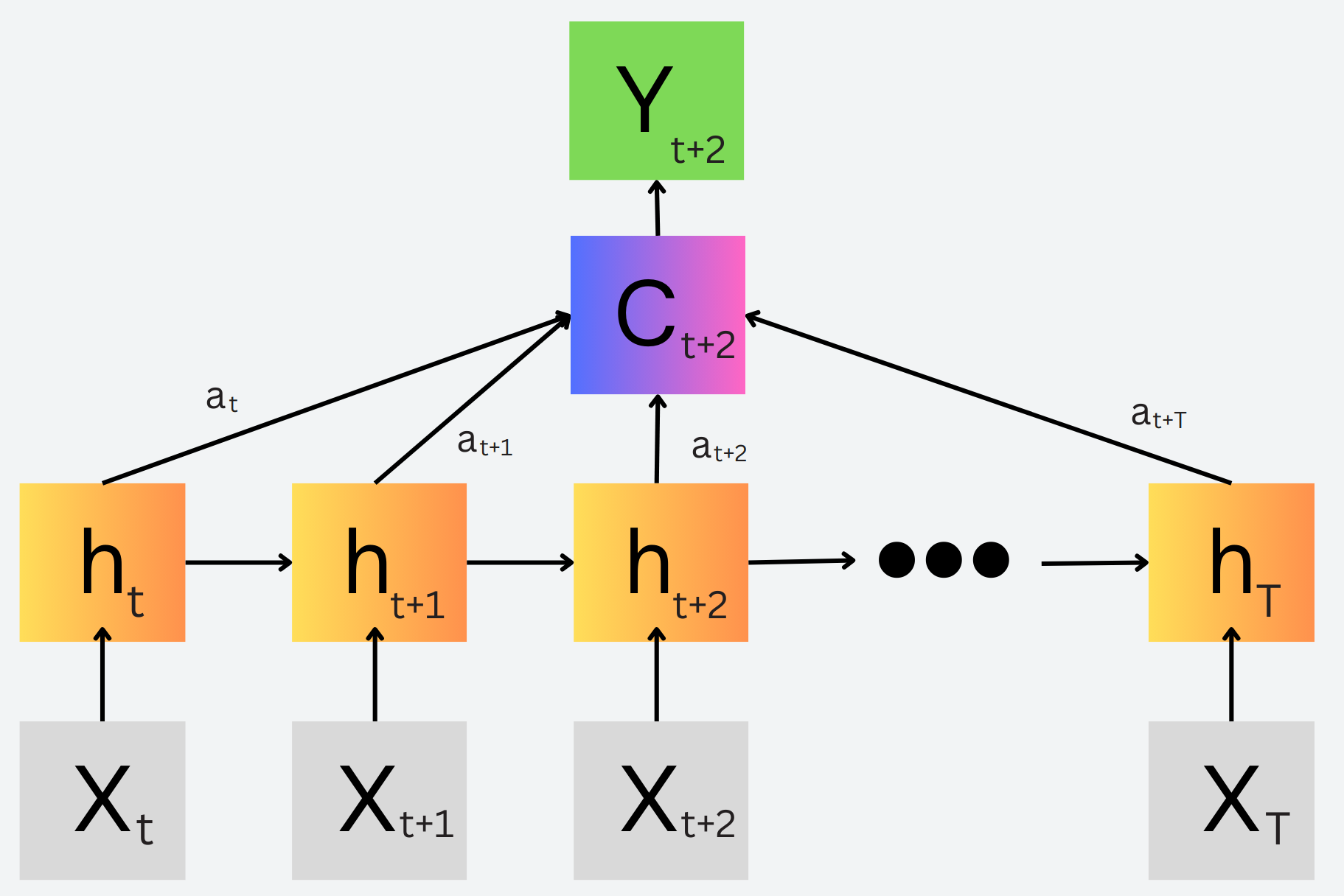
Now I keep saying weighted average, and this is because for one of the timesteps, the model has to learn the weights of what is the most important information to know at those times, and then weight them higher. As per the paper, the weights were learned through an alignment model, which was just a feedforward network that scores how well hidden states as time \(t\) is related to those around it in the sequence. These scores were then passed through a softmax to ensure all the learned weights sum up to 1, and then the context vectors are computed based on them. This means every context vector is a customized weighted average that learned exactly what information to put empahsis on at every timestep of the context vectors.
Problems#
There are some issues with this approach, however, some which were already known about RNNs:
Efficient but Slow: The RNN mechanism has a for-loop through the sequence making training very slow, but inference was efficient
Lack of Positional Information: Our context vectors are just weighted averages of hidden states, there is no information about position or time. In most sequence tasks, the order in your data appears is very important
Redundancy: We are effectively learning the same information twice - the hidden states encode sequential information, but the attention mechanism also encodes sequential information
Attention is All You Need!#
The groundbreaking paper, Attention is All You Need solved all of the problems above, but added a new one: computational cost. Lets first look at what the Attention Mechanism proposed in this paper is doing.
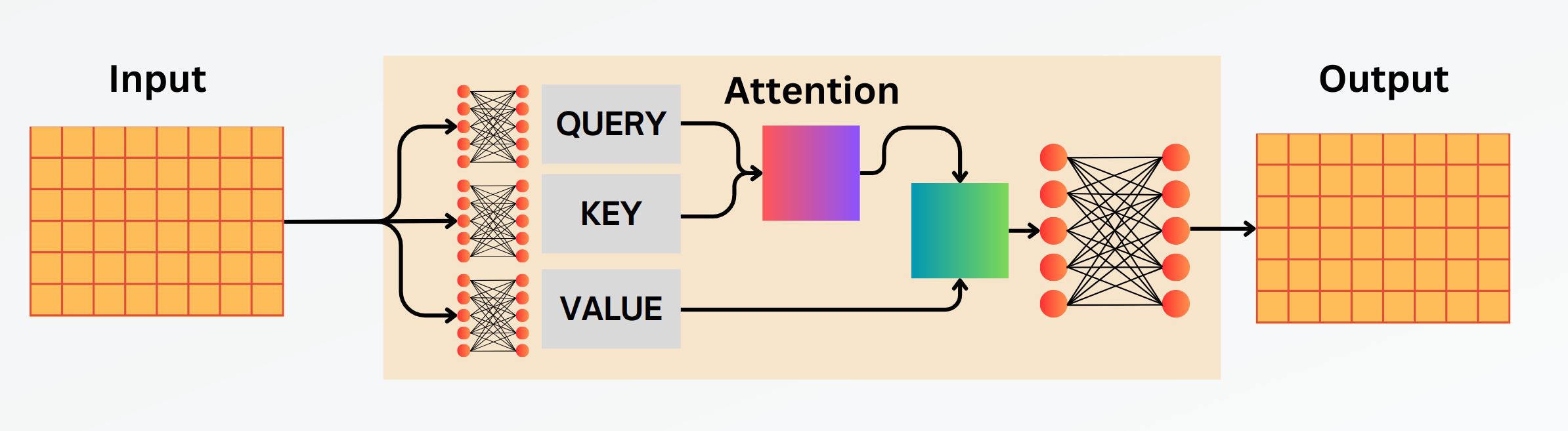
The input is a sequence of embedding vectors and the output is a sequence of context vectors. The three linear layers which you see in the above image take three things as an input — “QUERY, KEY & VALUE”. Let’s take a simple example to understand them.
If you were to search for something on Youtube or Google, The text which you type in the search box is the QUERY. The results which appear as the video or article title are the KEY and the content inside them is the VALUE. To find the best matches, the Query has to find the similarity between it and the Keys.
Lets quickly look at the formulation for this:
We see some new notation show up now: \(Q\), \(K\), \(V\). We introduce the concept of a token, which in the context of transformer models, is the basic, discrete unit of data. For LLMs, a token can be a word, part of a word (subword), or character. In other domain applications of transformers they can be other types of data elements, such as particle properties in particle physics.
Now we define \(Q\), \(K\), \(V\):
\(Q\): Queries, they are the token we are interested in
\(K\): Keys, they are the other tokens we want to compare our query against
\(V\): Values, they are the values we will weight in our weighted average
This is a little weird so lets step through it! First important note, the \(Q\), \(K\), and \(V\) are three projections of our original data input \(X\). This basically means we have three linear layers that all take the same input \(X\) to produce our \(Q\), \(K\), \(V\).
Step 1: Compute the Attention Matrix#
The first step is computing the Attention Matrix with \(Softmax(QK^T)\), where Q and K both have the shape Sequence Length x Embedding Dimension. The output of this computation will be Sequence Length x Sequence Length. This is what it looks like:
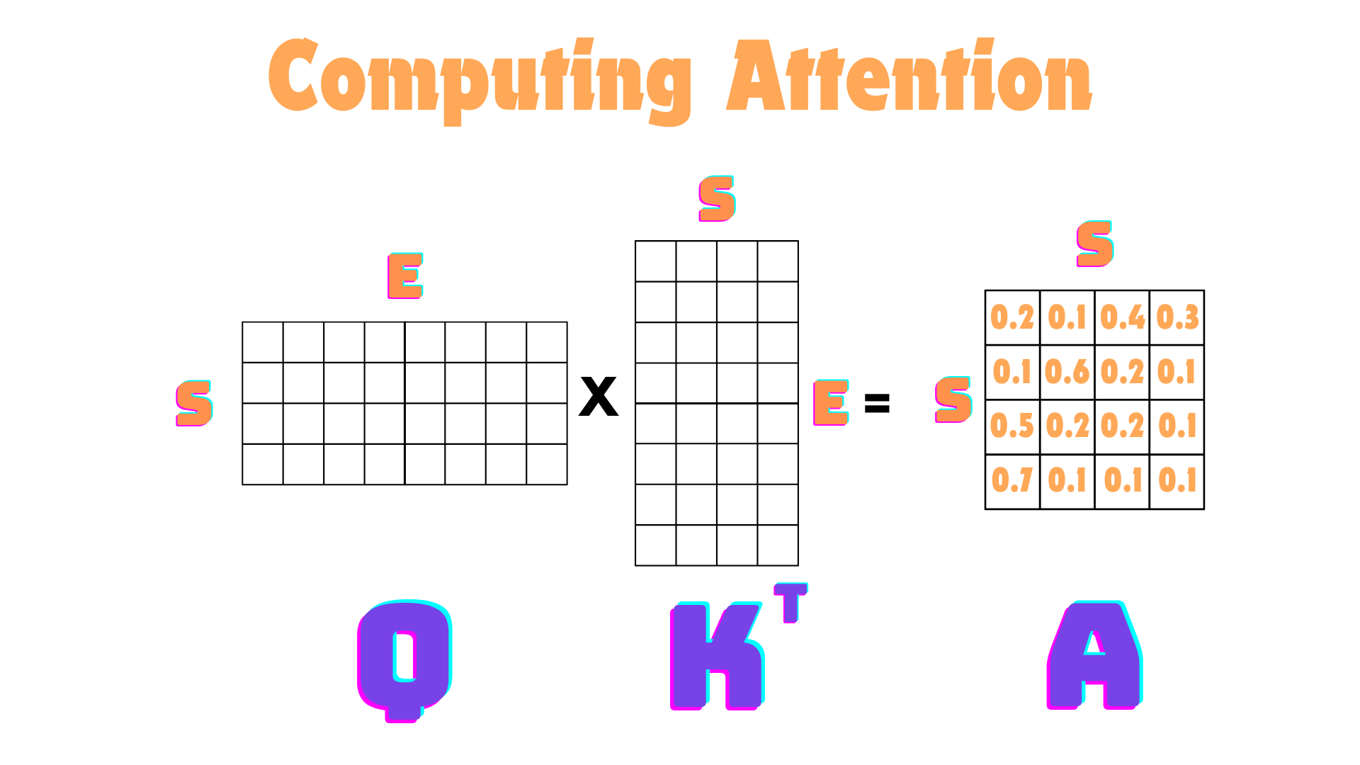
In the image above, I also applied the softmax (not shown for simplicity), so each row of the attention matrix adds up to 1 (like probabilities).
Recap: The Dot Product#
As a quick reminder, this whole mechanism depends on the dot product, and more specifically, its geometric interpretation
What the dot product really signifies is the similarity between vectors. Remember the cosine of 0 is just 1, so the highest possible cosine value would be when the vectors \(a\) and \(b\) point in the exact same direction. This means vectors that are similar in direction have higher magnitude.
Recap: Matrix Multiplication#
Also remember, matrix multiplication is basically just a bunch of dot products, repeating the multiply/add operation repeatedly. If we are multiplying matrix \(A\) with matrix \(B\), what we are really doing is doing the dot product of every row of \(A\) and every column of \(B\).
So with our quick recaps, lets go back to the image above, when we are multiplying \(Q\) by \(K^T\), we are multiplying each vector in the sequence \(Q\) by each vector in the sequence \(K\) and computing their dot product similarity. Again, \(Q\) and \(K\) are just projections of the original data \(X\), so really we are just computing the similarity between every possible combination of timesteps in \(X\). We also could have just done \(XX^T\), this would technically be the same thing, but by including the projections of \(X\) rather than using the the raw inputs themselves, we allow the model to have more learnable parameters so it can futher accentuate similarities and differences between different timesteps!
The final result of this operation is the attention matrix, that computes the similarity between every possible pairs of tokens.
Note: I didn’t say anything about the \(\frac{1}{\sqrt{d_e}}\) term in the formula. This is just a normalization constant that ensures our variance of the attention matrix isn’t too large after our matrix multiplication. This just leads to more stable training.
Step 2: Weighting the Values Matrix#
Now that we have the similarities of how each timestep is related to all the other timesteps, we can do our weighted average. After the weighted average computation, each vector for each timestep isn’t just the data of the timestep but rather a weighted average of all the vectors in the sequence and how they are related to that timestep of interest.
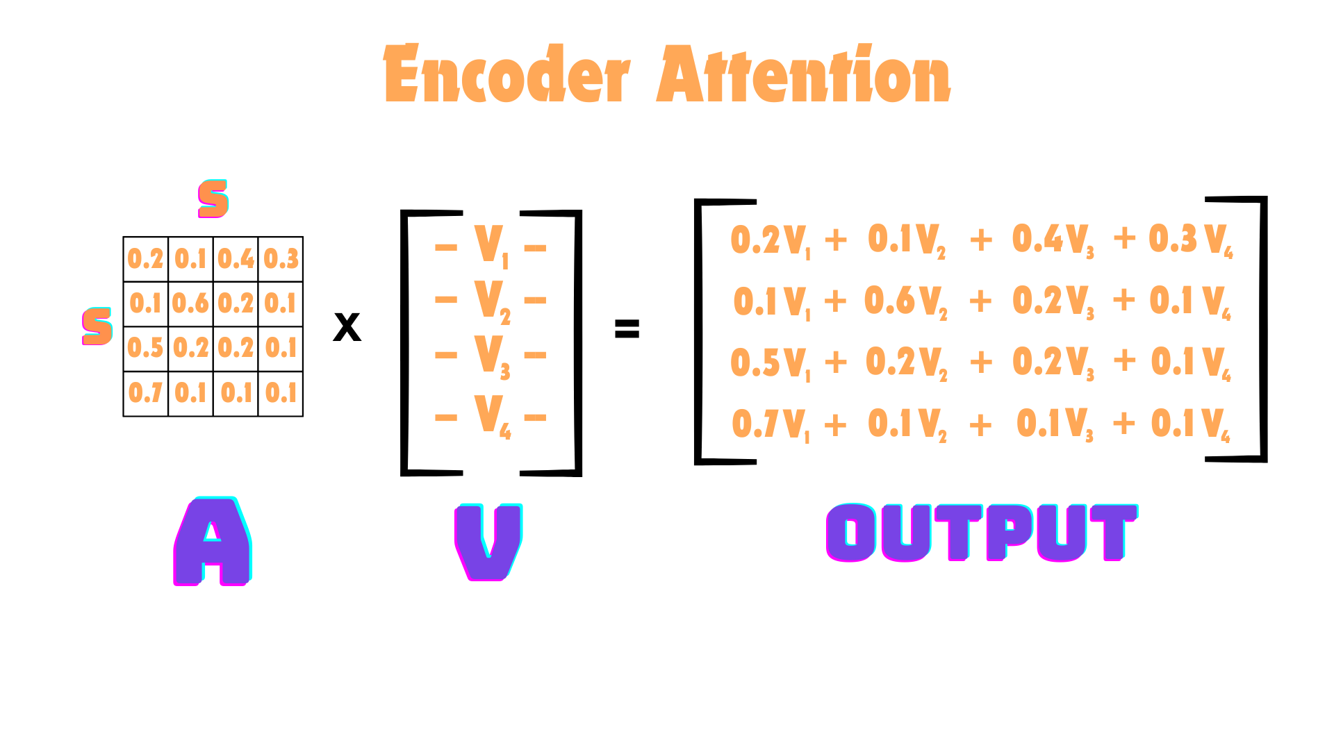
The output of this operation gives us the sequence of context vectors.
Enforcing Causality#
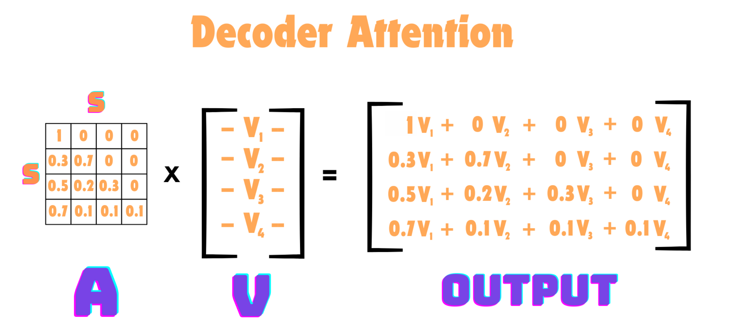
What we have seen so far is the equivalent to a Bidirectional RNN. The weighted average operation we are doing is between a timestep of interest and all timesteps before and after it. If we wanted a causal model, where a context vector only depends on the timesteps before it, then we need to apply a causal mask to our attention mechanism.
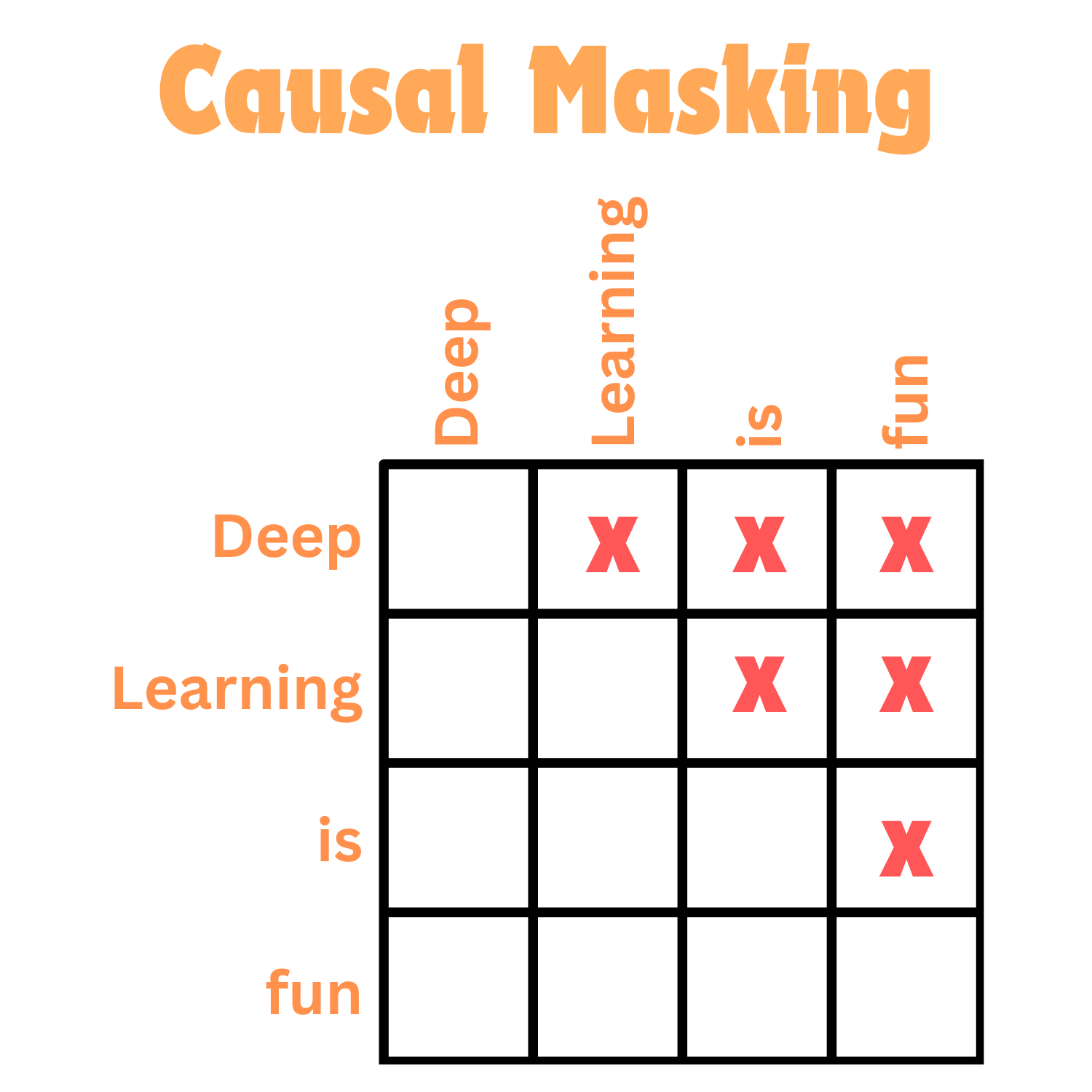
As you can see, we apply a mask to all values of \(t\) where the index of the column values (our key index) is greater than the index of the row value (our value index). In practice, once we apply this mask to our attention matrix, we can then multiply by our values. You will see that the context vector at time \(t\) is only then dependent on previous timesteps, as we make sure future vectors of \(V\) are zeroed out.
Lets Build This!#
Now that we have everything we need, we can build it! We wont be trainig any models now, just defining and exploring the architecture here. To do so, we will define some data in the form of Batch x Sequence Length x Embed Dim. The Embedding dimension is the dimension of the vector we want to use to represent a single timestep, and the sequence length is how many timesteps there are in total.
import torch
import torch.nn as nn
import torch.nn.functional as F

### Lets Define some Random Data ###
batch_size = 4
sequence_length = 64
embed_dim = 128

x = torch.randn(batch_size, sequence_length, embed_dim)
print("Shape of Input is:", x.shape)
Shape of Input is: torch.Size([4, 64, 128])
Implement Attention Without Any Learnable Parameters#
This whole attention operation is again very flexible and there is technically no reason to have any learnable parameters in its formulation (other than the obvious for wanting better predictive performance). So lets quickly just implement the formula as is using raw inputs \(X\) rather than doing any learned projections of the data.
Step 1
Compute \(XX^T\) which will provide the similarity score between every pair of vectors in \(X\). This will be contained inside a batch x sequence_length x sequence_length matrix
Step 2
After computing the similarity score, we can check and see that the variance of the similarity matrix is extremely high. This is the main reason for the normalization of dividing by the square root of the embedding dimension. In the end, the similarity scores are passed through a Softmax to compute a probability vector, dividing by a constant basically acts as a temperature parameter to cool the distribution and provide more stable training.
Step 3
Each row of our sequence_length x sequence_length matrix is the similarity of how one timestep is related to all other timesteps. Instead of raw similarity scores, we will convert them to probabilities, so that when we do the weighted average on our values matrix, the weights add up to 1.
### First compute XX^T for similarity score between every pair of tokens ###
similarity = (x @ x.transpose(1,2))

### Normalize the Similarity Scores ###
print("Prenormalization Variance:", similarity.var())
similarity_norm = similarity / (embed_dim**0.5)
print("Normed Similarity Variance:", similarity_norm.var())

### Check the Shape of our Similarity Tensor ###
print("Shape of Normed Similarity:", similarity_norm.shape)

### Compute similarity on every row of the attention matrix (i.e along the last dimension) ###
attention_mat = similarity_norm.softmax(dim=-1)

### Verify each row adds up to 1 ###
summed_attention_mat = attention_mat.sum(axis=-1)
print("Everything Equal to One:", torch.allclose(summed_attention_mat, torch.ones_like(summed_attention_mat)))

### Multiply our Attention Matrix against its Values (X in our case) for our Weighted Average ###
context_vectors = attention_mat @ x

print("Output Shape:", context_vectors.shape)
Prenormalization Variance: tensor(388.4557)
Normed Similarity Variance: tensor(3.0348)
Shape of Normed Similarity: torch.Size([4, 64, 64])
Everything Equal to One: True
Output Shape: torch.Size([4, 64, 128])
Thats it! This is basically all the attention computation is doing mathematically, we will add in the learnable parameters in just a bit. Something important to bring to your attention is the input shape of \(x\) and our output shape of the context vectors are identical. Again, the input is the raw data, the output is weighted averaged of how every token is realted to all the other ones. But the shapes not changing is quite convenient, and allows us to stack together a bunch attention mechanisms on top of one another!
Lets Add Learnable Parameters#
This time, instead of using \(X\) as our input, we will create our three projections of \(X\) (Queries, Keys and Values) and then repeat the operation we just did. Also for convenience, we will wrap it all in a PyTorch class so we can continue adding stuff onto it as we go on to build up a general attention block.
Now what are these projections exactly? The are pointwise (or per timestep) projections! Remember, in our example here, each timestep is encoded by a vector of size 128. We will create three learnable weight matricies, incorporated inside the Linear modules in PyTorch, that take these 128 numbers per timestep and projects them to another 128 numbers (it is typical to keep the embedding dimension the same). This is a per timestep operation not across timesteps operation (across timesteps occurs within the attention computation). Obviously, PyTorch will accelerate this per timestep operation by doing it in parallel, but regardless, different timesteps dont get to see each other in the projection step.
class Attention(nn.Module):
    def __init__(self, embedding_dimension):
        super().__init__()

        self.embed_dim = embedding_dimension

        ### Create Pointwise Projections ###
        self.query = nn.Linear(embedding_dimension, embedding_dimension)
        self.key   = nn.Linear(embedding_dimension, embedding_dimension)
        self.value = nn.Linear(embedding_dimension, embedding_dimension)

    def forward(self, x):

        ### Create Queries, Keys and Values from X ###
        q = self.query(x)
        k = self.key(x)
        v = self.value(x)

        ### Do the same Computation from above, just with our QKV Matricies instead of X ###
        similarity = (q @ k.transpose(1,2)) / (self.embed_dim ** 0.5)
        attention = similarity.softmax(axis=-1)
        output = attention @ v

        return output

attention = Attention(embedding_dimension=128)
output = attention(x)
print(output.shape)
torch.Size([4, 64, 128])
MultiHeaded Attention#
Now we have a small problem. Remember, the Attention matrix encodes the similarity between each pair of timesteps in your sequence. But in many cases, language being a prime example, there can be different types of relationships between different pairs of words, but our attention computation is restricted to learn only one of them. The solution to this is Multi Headed Attention. Inside each attention computation, what if we have 2 attention matricies, or 8 or however many we want! The more we have the larger diversity of relationships we can learn!
Single Headed Attention Recap#
Lets summarize everything we have seen so far with a single visual, and we will call this a Single Head of attention. We will also have our embedding dimension for each word in the sequence be 9, and the sequence length is 8.
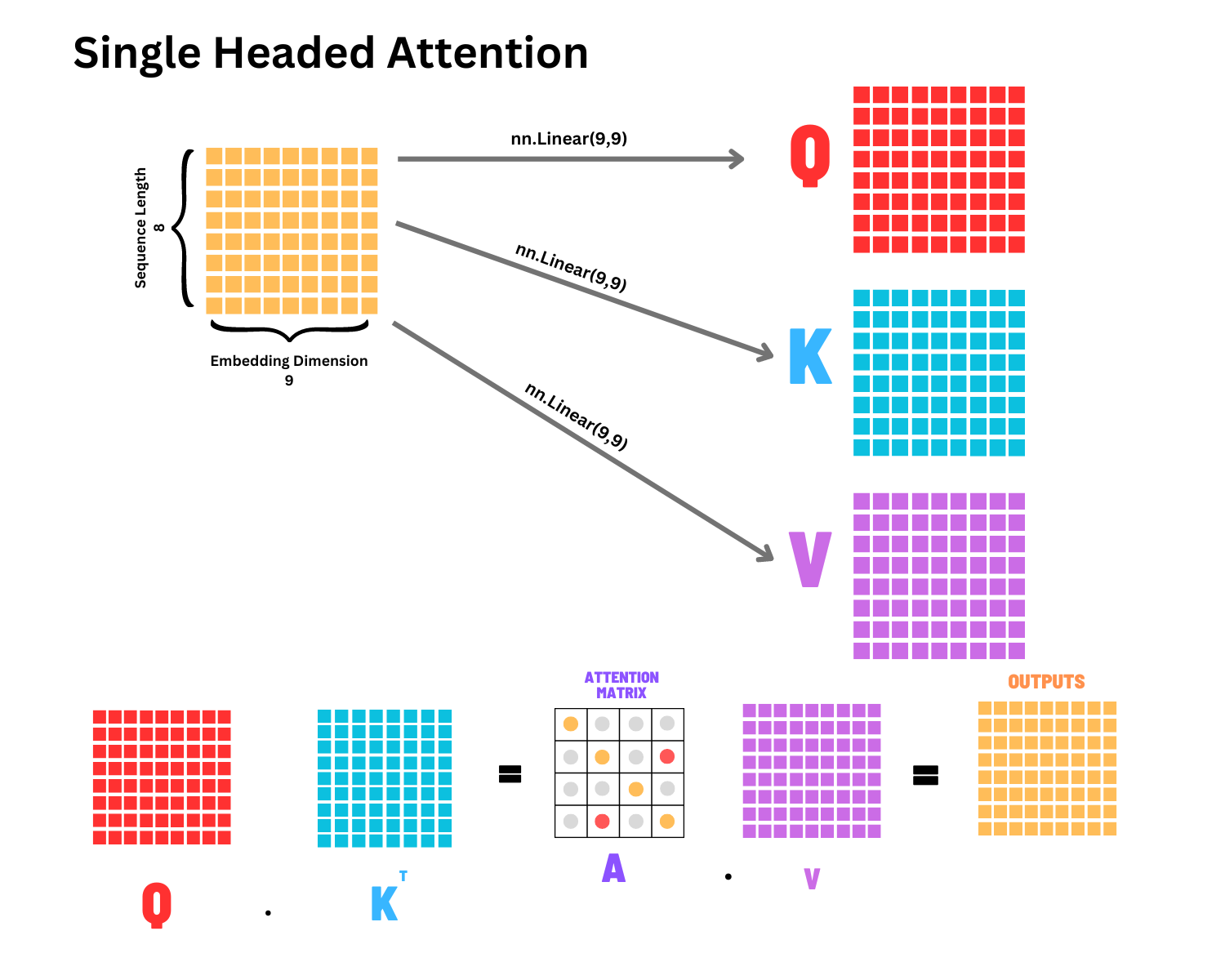
This is again called single headed attention because we only compute a single attention matrix following the logic described above.
Moving to MultiHeaded Attention#
For multiheaded attention there isn’t really a lot changing. Remember, to create our \(Q\), \(K\), \(V\) in single headed attention, we have 3 linear projection layers that take in the embedding dimension and output the same embedding dimension (in our case it takes in 9 and outputs 9). But in multiheaded attention, we can actually reduce our embedding dimension to a smaller value, do the attention computation on the tokens with this condensed embedding dimension, repeat it a bunch of times, and then concatenate together the outputs.
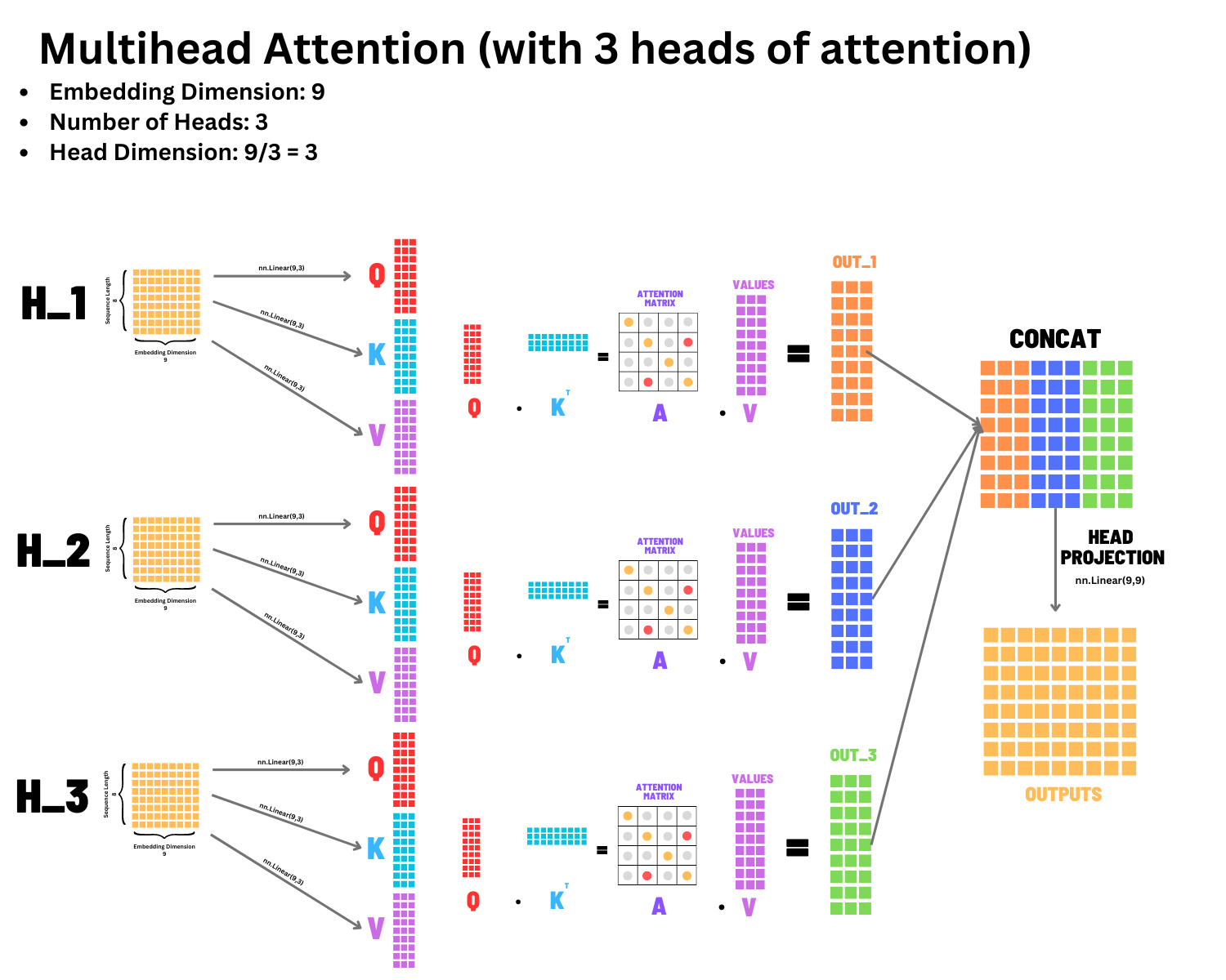
It is general practice to have the number of heads you pick to be a divisor of the embedding dimension. For example, in our case, our original embedding dimension is 9, so we can pick 3 heads because 9 is divisible by 3. This also means our head dimension would now be 3, because 9/3 = 3. In typical transformers, the embedding dimension is 768, and they typically have 12 heads of attention. This means each head of attention will have a dimension of 64 because 768/12 = 64.
The main reason we want it to evenly divide is because we have three heads, each takes in an embedding dimension of 9 and compresses to 3 before computing attention, and then outputs a tensor of embedding size 3. We can then take our 3 tensors, each having an embedding dimension of 3, concatenate them together, returning us back to the 9 that we began with! Again, this is just for convenience, so the embedding dimension of the input and output tensor dont change in any way.
The last problem is that since each head of attention is computed individually, the final concatenated tensor has a bunch of heads of attention packed together, but we never got to share information between the different heads of attention. This is why we have the final head projection, that will take in the embedding dimension of 9 from our concatenated tensor, and output an embedding dimension of 9, therefore meshing information across the heads of our embedding dimension.
Lets go ahead and build this module as shown in the figure above. Each head will have 3 projection layers for \(Q\),\(K\),\(V\). We will perform the attention computation and then stick all the results back together at the end.
class MultiHeadAttention(nn.Module):
    def __init__(self, embedding_dimension, num_heads):
        super().__init__()

        ### Make sure Embedding Dimension is Divisible by Num Heads ###
        assert embedding_dimension % num_heads == 0, f"Make sure your embed_dim {embedding_dimension} is divisible by the number of heads {num_heads}"

        self.embed_dim = embed_dim
        self.num_heads = num_heads

        ### Compute Head Dimension ###
        self.head_dim = self.embed_dim // self.num_heads


        ### Create a List of Lists which has all our Q,K,V projections for each head ###
        self.multihead_qkv = nn.ModuleList()

        ### For head Head create the QKV ###
        for head in range(self.num_heads):

            ### Create a dictionary of the 3 projection  layers we need ###
            qkv_proj = nn.ModuleDict(
                [
                    ["Q", nn.Linear(self.embed_dim, self.head_dim)],
                    ["K", nn.Linear(self.embed_dim, self.head_dim)],
                    ["V", nn.Linear(self.embed_dim, self.head_dim)],
                ]
            )

            ### Store Dictionary in List ###
            self.multihead_qkv.append(qkv_proj)

        ### Create final Projection layer, it will be applied to the concatenated heads will have shape embed_dim again ###
        self.head_mesh = nn.Linear(self.embed_dim, self.embed_dim)

    def forward(self, x):

        ### Create a list ot store each heads output ###
        head_outs = []

        ### Loop Through Each head of Attention ###
        for head in self.multihead_qkv:

            ### Access layers like a dictionary (ModuleDict) ###
            ### q,k,v will be (Batch x Seq len x head_dim)
            q = head["Q"](x)
            k = head["K"](x)
            v = head["V"](x)

            ### Now do the same Attention computation as before! ###
            similarity = (q @ k.transpose(1,2)) / (self.embed_dim ** 0.5)
            attention  = similarity.softmax(axis=-1)
            output = attention @ v

            ### Store this output in the head_outs ###
            head_outs.append(output)

        ### head_outs has num_heads tensors, each with the compressed embedding dimension of head_dim ###
        ### We can concatenate them all back together along the embedding dimension just like we did in the image above ###
        head_outs = torch.cat(head_outs, dim=-1)

        ### head_outs will have the same shape now as our input x! ###
        if head_outs.shape != x.shape:
            raise Exception("Something has gone wrong in the attention computation")

        ### Now each head was computed independently, we need them to get to know each other, so pass our head_outs through final projection ###
        output = self.head_mesh(head_outs)

        return output


embed_dim = 9
num_heads = 3
seq_len = 8
mha = MultiHeadAttention(embed_dim, num_heads)

### Create a random tensor in the shape (Batch x Seq Len x Embed Dim) ###
rand = torch.randn(3,seq_len,embed_dim)

### Pass through MHA ###
output = mha(rand)
Increasing Efficiency#
We now have successfully implemented a Multi Head Attention layer! This has all the same math and lodgic of attention, except for one small issue: efficiency. Typically we want to avoid for loops as much as possible in our PyTorch code, being able to vectorize and do things in parallel will make much better use of the GPUs we train on. To make this more efficient, there is something we need to understand first: PyTorch Linear layers on multidimensional tensors.
Linear Layers on MultiDimensional Tensors#
We have already seen nn.Linear(input_dim, output_dim) many times already, and this module expects a tensor of shape [Batch x input_dim] and it will output [Batch x output_dim]. But what if our input is [Batch x Dim1 x Dim2 x input_dim], then what happens? Basically, PyTorch will automatically flatten all the dimensions other than the last one automagically, do the Linear layer, and then return back to the expected shape, so we would get an output of [Batch x Dim1 x Dim2 x output_dim]. Another way of thinking about this is, PyTorch linear layers only are applied to the last dimension of your tensor.
Lets do a quick example:
fc = nn.Linear(10,30)

tensor_1 = torch.randn(5,10)
tensor_1_out = fc(tensor_1)
print("Input Shape:", tensor_1.shape, "Output Shape:", tensor_1_out.shape)

tensor_2 = torch.randn(5,1,2,3,4,10)
tensor_2_out = fc(tensor_2)
print("Input Shape:", tensor_2.shape, "Output Shape:", tensor_2_out.shape)
Input Shape: torch.Size([5, 10]) Output Shape: torch.Size([5, 30])
Input Shape: torch.Size([5, 1, 2, 3, 4, 10]) Output Shape: torch.Size([5, 1, 2, 3, 4, 30])
Packing Linear Layers#
Another important idea is packing our Linear layers together. Lets think about our Multi Head example again: each projection for Q, K and V have a Linear layer that takes in 9 values and outputs 3 values, and we repeat this 3 times for each head. Lets just think about our Queries for now.
Query for Head 1: Take in input \(x\) with embedding dim 9 and outputs tensor with embedding dimension 3
Query for Head 2: Take in input \(x\) with embedding dim 9 and outputs tensor with embedding dimension 3
Query for Head 3: Take in input \(x\) with embedding dim 9 and outputs tensor with embedding dimension 3
Well what if we reframed this? What if we had a single Linear layer that takes input \(x\) with embedding dim 9 and outputs something with embedding dim 9. Afterwards, we can cut the matrix into our three heads of attention. Lets do a quick example:
tensor = torch.randn(1,8,9)
fc = nn.Linear(9,9)

### Pass tensor through layer to make Queries ###
q = fc(tensor)
print("Shape of all Queries:", q.shape)

### Cut Embedding dimension into 3 heads ###
q_head1, q_head2, q_head3 = torch.chunk(q, 3, axis=-1)
print("Shape of each Head of Query:", q_head1.shape)
Shape of all Queries: torch.Size([1, 8, 9])
Shape of each Head of Query: torch.Size([1, 8, 3])
MultiDimensional Matrix Multiplication#
So, we have composed our 9 Linear layers (3 heads have 3 projections for \(Q\), \(K\), \(V\) each) into just 3 Linear layers, where we have packed all the heads into them. But after we chunk up our \(Q\), \(K\), \(V\) tensors each into three more tensors for each head we will still need to do the looping operation to go through the cooresponding \(q\), \(k\), \(v\) matricies. Can we parallelize this too? Of course! We just need to better understand higher dimensional matrix multiplication.
Recap#
Matrix multiplication is typicall seen like this, multiplying an [AxB] matrix by a [BxC] which will produce a [AxC] matrix. But what if we have a [Batch x dim1 x A x B] multiplied by a [Batch x dim1 x B x C]. Matrix multiplication again only happens on the last two dimensions, so because our first tensor ends with an [AxB] and the second tensor ends with a [BxC], the resulting matrix multiplication will be [Batch x dim1 x A x C. Lets see a quick example:
a = torch.randn(1,2,6,4)
b = torch.randn(1,2,4,3)
print("Final Output Shape:", (a@b).shape)
Final Output Shape: torch.Size([1, 2, 6, 3])
The Trick of Parallelizing Heads#
Now for the trick of parallelizing our heads by using everything we have just seen. All we need to do is split the embedding dimension up and move the heads out of the way so the computation can occur. Remember, we have our \(Q\), \(K\), and \(V\) matricies right now that each contain all the projected heads and are in the shape [Batch x Seq_len x Embed_dim] ([batch x 8 x 9] in our case).
The first step is to split the embedding dimension into the number of heads and head dimension. We already know that our embedding dimension is divisible as thats how we set it, so we can do
[Batch x Seq_len x Embed_dim]->[Batch x Seq_len x Num_Heads x Embed_Dim]. (This would be taking our [batch x 8 x 9] and converting to [batch x 8 x 3 x 3] in our case).The attention computation has to happen between two matricies of shape
[Seq_len x Embed_Dim]for queries and[Embed_Dim x Seq_len]for our transposed keys. In the case of multihead attention, the matrix multiplication happens across the Head Dimension rather than embedding. If our Queries, Keys and Values are in the shape[Batch x Seq_len x Num_Heads x Embed_Dim], we can just transpose the Seq_len and Num_heads dimensions and make a tensor of shape[Batch x Num_Heads x Seq_len x Embed_Dim]. This way when I do Queries multiplied by the Transpose of Keys I will be doing[Batch x Num_Heads x Seq_len x Embed_Dim]multiplied by[Batch x Num_Heads x Embed Dim x Seq Len]creating the attention matrix[Batch x Num_Heads x Seq_len x Seq Len]. Therefore we have effectively created for every sample in the batch, and for every head of attention, a unique attention matrix! Thus we have parallelized the Attention Matrix computation.Now that we have all of our attention matricies
[Batch x Num_Heads x Seq_len x Seq Len], we can perform our scaling by a constant, and perform Softmax across every row of each attention matrix (along the last dimension).The next step is to multiply our attention matrix
[Batch x Num_Heads x Seq_len x Seq Len]by the Values which is in the shape[Batch x Seq_len x Num_Heads x Embed_Dim], which will get us to[Batch x Num_Heads x Seq_len x Embed_Dim]!Lastly, we need to put our Num Heads and Embedding dimensions back together, so we can permute the Num Heads and Seq Len dimensions again which gives us
[Batch x Seq_len x Num_Heads x Embed_Dim]and flatten on the last two dimension finally giving us[Batch x Seq_len x Num_Heads x Embed_Dim].This flattening operation is equivalent to concatenation of all the heads of attention, so we can pass this through our final projection layer so all the heads of attention gets to know each other!
More Efficient Attention Implementation#
We will also include some extra dropout layers typically added to attention computations.
class SelfAttentionEncoder(nn.Module):
    """
    Self Attention Proposed in `Attention is All  You Need` - https://arxiv.org/abs/1706.03762
    """

    def __init__(self,
               embed_dim=768,
               num_heads=12,
               attn_p=0,
               proj_p=0):
        """

        Args:
            embed_dim: Transformer Embedding Dimension
            num_heads: Number of heads of computation for Attention
            attn_p: Probability for Dropout2d on Attention cube
            proj_p: Probability for Dropout on final Projection
        """

        super(SelfAttentionEncoder, self).__init__()

        ### Make Sure Embed Dim is Divisible by Num Heads ###
        assert embed_dim % num_heads == 0
        self.num_heads = num_heads
        self.head_dim = int(embed_dim / num_heads)

        ### Define all our Projections ###
        self.q_proj = nn.Linear(embed_dim, embed_dim)
        self.k_proj = nn.Linear(embed_dim, embed_dim)
        self.v_proj = nn.Linear(embed_dim, embed_dim)
        self.attn_drop = nn.Dropout(attn_p)

        ### Define Post Attention Projection ###
        self.proj = nn.Linear(embed_dim, embed_dim)
        self.proj_drop = nn.Dropout(proj_p)

    def forward(self, x):

        batch, seq_len, embed_dim = x.shape

        ### Compute Q, K, V Projections,and Reshape/Permute to [Batch x Num Heads x Seq Len x Head Dim]
        q = self.q_proj(x).reshape(batch, seq_len, self.num_heads, self.head_dim).transpose(1,2).contiguous()
        k = self.k_proj(x).reshape(batch, seq_len, self.num_heads, self.head_dim).transpose(1,2).contiguous()
        v = self.v_proj(x).reshape(batch, seq_len, self.num_heads, self.head_dim).transpose(1,2).contiguous()

        ### Perform Attention Computation ###
        attn = (q @ k.transpose(-2,-1)) * (self.head_dim ** -0.5)
        attn = attn.softmax(dim=-1)
        attn = self.attn_drop(attn)
        x = attn @ v

        ### Bring Back to [Batch x Seq Len x Embed Dim] ###
        x = x.transpose(1,2).reshape(batch, seq_len, embed_dim)

        ### Pass through Projection so Heads get to know each other ###
        x = self.proj(x)
        x = self.proj_drop(x)

        return x

embed_dim = 9
num_heads = 3
seq_len = 8
a = SelfAttentionEncoder(embed_dim, num_heads)

### Create a random tensor in the shape (Batch x Seq Len x Embed Dim) ###
rand = torch.randn(3,seq_len,embed_dim)

### Pass through MHA ###
output = a(rand)
print("Final Output:", output.shape)
Final Output: torch.Size([3, 8, 9])
Padding#
One aspect we haven’t talked about yet is padding. We have to train in batches, and unfortunately, if each sequence is of different lengths, we cannot put them together simply and dynamically, In this situation, we just take all the sequences that are shorter than the longest one in the batch and then pad them.
Sequence Padding and Attention Masking#
One typical consideration for models like this is, when we pass in sentences of data, different sentences have different lengths. To create a matrix of tokens, we need to make sure all the sequences are the same, therefore we have to pad the shorter sequences to the longer ones. This is what the padding looks like:
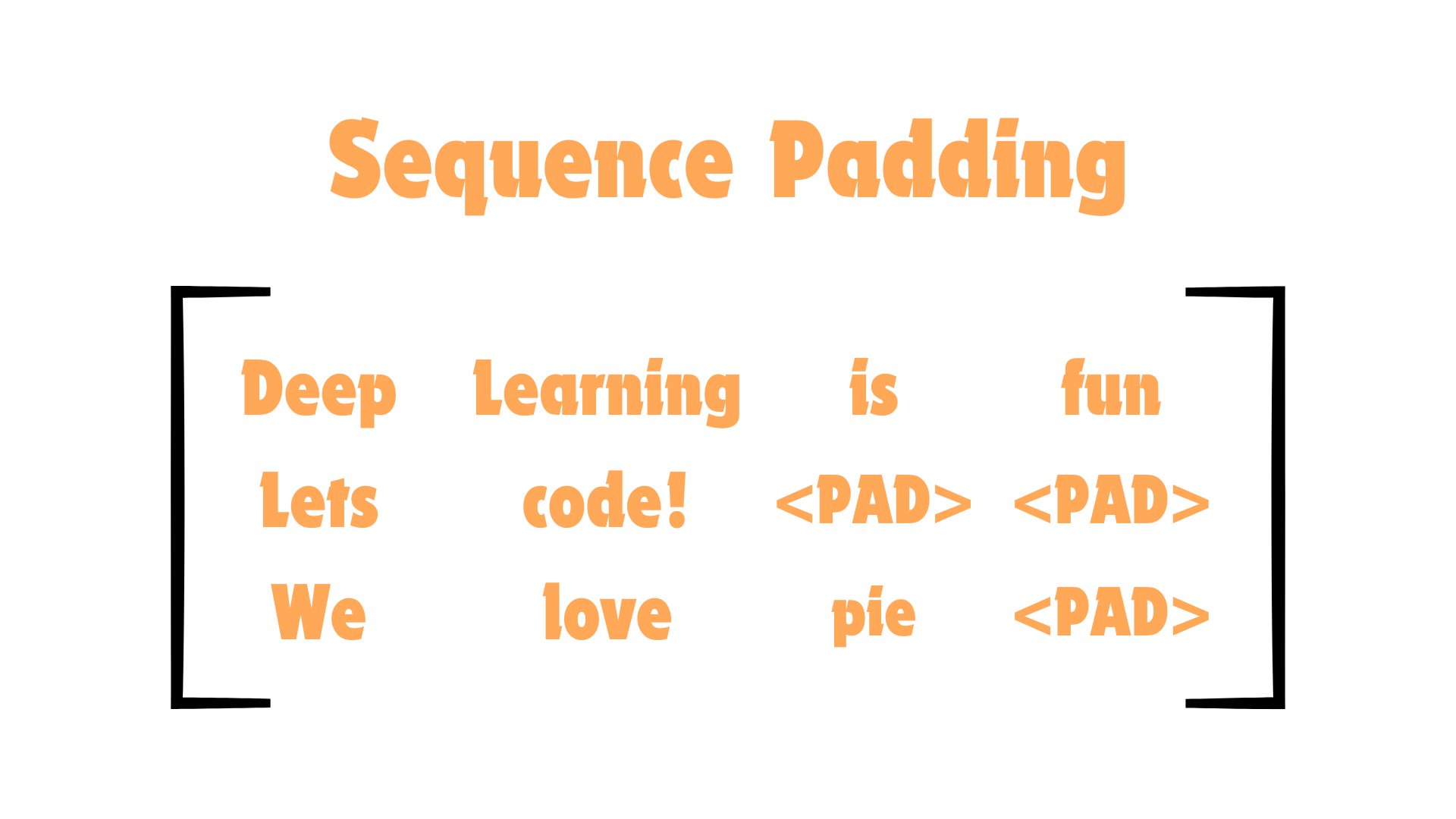
The pad tokens are just fillers and they don’t add any information at all to the data. To deal with this, we need to make sure that when we compute attention, these pad tokens are ignored. This is very similar to the Causal Mask in GPT, and we will be doing exactly what we did there, fill in the masked locations with \(-\infty\) before Softmax is computed. Lets take a quick look at this for one of the sentences above.
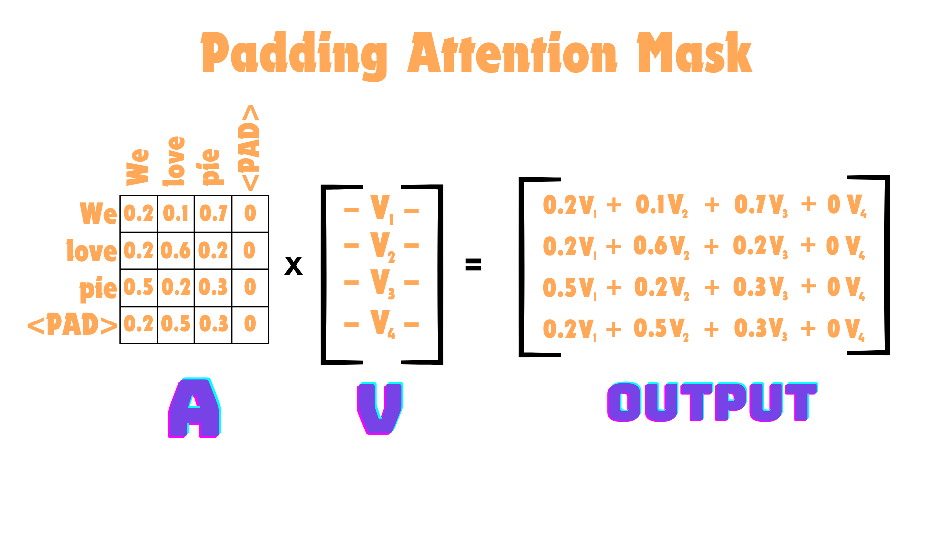
You can see that we zero out the columns of our attention mask that has padding tokens, but not the row. The reason for this is, the model should learn the relation of how the padding tokens are related to the words (this is most likely just positional information that padding is at the end), but it should not learn how other words are related to padding, as the padding adds no semantic meaning. This is why, when multiplying by our values, we have zeroed out the attention weights of the 4th column, as when computing weighted averages of how one word is related to all others, the padding token is not included.
Computing the Reweighted Padded Attention Mask#
Lets create some numbers so we can get a better idea of how this works. Let the tokens be \(X = [10, 2, \text{<pad>}]\), so the third token is a padding token. Lets then also pretend, we pass this to our model, and when we go to compute our attention \(QK^T\). The raw output before the Softmax is below:
Remember, the equation for softmax is:
If we ignore padding and everything right now, we can compute softmax for row of the matrix above:
But what we need is to mask out all the tokens in this matrix related to padding. Just like we did in GPT, we will fill in the indexes of the that we want to mask with \(-\infty\). If only the last token was a padding token in our sequence, then the attention before the softmax should be written as:
Taking the softmax of the rows of this matrix then gives:
Which is exactly what we want! Therefore, when computing attention, we need to know which tokens are padding tokens in our data, and then go ahead and perform this computation on our attention output before multiplying with values.
Add Padding to our Attention Computation#
There are a few ways to indicate padding, but the most common is a simple True/False vector. Lets say we have the following 3 sequences:
sequence_1: [a1, a2, a3]
sequence_2: [b1, b2, b3, b4]
sequence_3: [c1, c2, c3]
In this situation we would pad sequence_1 and sequence_3 to the longest sequence, so after padding we would have something like this:
sequence_1: [a1, a2, a3, <PAD>]
sequence_2: [b1, b2, b3, b4]
sequence_3: [c1, c2, c3, <PAD>]
Now we will create boolean vectors, identifying True/False for tokens we want to compute attention on. Anything that is a <PAD> token would be omitted, so we would have the following attention masks for each sequence:
sequence_1: [
True,True,True,False]sequence_2: [
True,True,True,True]sequence_3: [
True,True,True,False]
Then, as indicated above, for columns for tokens identified as False (because they are pad tokens) we will zero out the attention scores and reweight them to properly compute attention without learning how words are related to the padding (only how the padding is related to the words)
Repeating to Match Attention Matrix Shape#
So we now have our attention mask and know we need to mask the columns in our attention matrix that coorespond to them. Lets also pretend for now we are doing single headed attention, we can deal with the multiheaded attention in a bit. In this case, lets take a look at our attention and mask shapes:
attn.shape - (Batch x seq_len x seq_len)
mask.shape - (Batch x seq_len)
It is clear that our mask is missing a dimension, and we need to repeat it. Lets take sequence_1 for instance that has a mask of [True, True, True, False]. Because the sequence length here is 4, lets repeat this row 4 times:
By repeating our mask for sequence_1, we get exactly a seq_len x seq_len matrix where the column we don’t want to compute attention for is indicated by the False.
Therefore our final mask will be of shape Batch x seq_len x seq_len
CAVEAT: Technically we don’t need to do this, and this is why the padding can get confusing as different people/functions do it different ways. First of all, lets say we reshaped our attention mask from(Batch x seq_len to Batch x 1 x seq_len. That 1 is a dummy dimension, and when we use the Tensor.masked_fill_ it will automatically broadcast our attention mask across that dummy 1 dimension. On the other hand, when we go to use flash_attention at the end, this method wants the tensor specifically in the shape Batch x seq_len x seq_len.
For testing, lets just use a 1 x 6 x 6 tensor as a fake 8 x 8 attention matrix for a single sample (not multihead attention yet). Lets also pretend the last two tokens are pad tokens, so we want the attention mask that will fill the last two columns with \(-\infty\), so when we take the softmax in the future it’ll become zero!
Tensor.masked_fill_ will fill anywhere indicated as True with our fill value. In our case though, we have the tokens we don’t want to compute on (the ones we want to fill with \(-\infty\)) as false. So we just need to flip the boolean in our attention mask.
### Create an example attention matrix (b x n x n) ###
rand_attn = torch.rand(1,6,6)

### Create Attention Mask in the shape (b x n) ###
attention_mask = torch.tensor([1,1,1,1,0,0]).unsqueeze(0).bool()

print("Method 1:")
print("--------")
### Add Extra Dimension for the (b x n x n) ###
### So unsqueeze mask to be (b x 1 x n) ###
attention_mask = attention_mask.unsqueeze(1)

### Unsqueezed with dummy broadcast dimension ###
print(attention_mask)
print(rand_attn.masked_fill_(~attention_mask, float("-inf")))

print("Method 2:")
print("--------")
### Repeat the Dummy Dimension so attention mask is (b x n x n) ###
attention_mask = attention_mask.repeat(1,6,1) # repeat dummy middle dim 6 times (for the seq_len)
print(attention_mask)
print(rand_attn.masked_fill_(~attention_mask, float("-inf")))
Method 1:
--------
tensor([[[ True,  True,  True,  True, False, False]]])
tensor([[[0.4689, 0.9644, 0.5678, 0.0910,   -inf,   -inf],
         [0.3722, 0.4994, 0.9155, 0.3433,   -inf,   -inf],
         [0.5357, 0.1792, 0.9417, 0.2629,   -inf,   -inf],
         [0.2274, 0.2336, 0.0679, 0.9231,   -inf,   -inf],
         [0.0101, 0.5860, 0.8541, 0.9838,   -inf,   -inf],
         [0.8340, 0.5832, 0.5072, 0.5373,   -inf,   -inf]]])
Method 2:
--------
tensor([[[ True,  True,  True,  True, False, False],
         [ True,  True,  True,  True, False, False],
         [ True,  True,  True,  True, False, False],
         [ True,  True,  True,  True, False, False],
         [ True,  True,  True,  True, False, False],
         [ True,  True,  True,  True, False, False]]])
tensor([[[0.4689, 0.9644, 0.5678, 0.0910,   -inf,   -inf],
         [0.3722, 0.4994, 0.9155, 0.3433,   -inf,   -inf],
         [0.5357, 0.1792, 0.9417, 0.2629,   -inf,   -inf],
         [0.2274, 0.2336, 0.0679, 0.9231,   -inf,   -inf],
         [0.0101, 0.5860, 0.8541, 0.9838,   -inf,   -inf],
         [0.8340, 0.5832, 0.5072, 0.5373,   -inf,   -inf]]])
Matching Shapes for MultiHead Attention#
So we now have our attention mask and know how to mask the columns cooresponding to them. But we have one other problem: Multi Head Attention. This means we don’t have just a single attention matrix, but rather num_heads of them. This means we need to mask the corresponding columns of ALL attention matricies across the heads. Lets take a quick look at our tensors in question again:
attn.shape - (Batch x num_heads x seq_len x seq_len)
mask.shape - (Batch x seq_len)
This means we can do what we did earlier, just twice! We can take our mask and unsqueeze twice, and go from Batch x seq_len to Batch x 1 x 1 x seq_len, and this would be totally fine. Except again, when we do our flash_attention later, it again expects a seq_len x seq_len. Luckily though, flash attention will broadcast over the head dimension as long as that dimension is present in the mask, so we just have to do what we did earlier and repeat Batch x 1 x 1 x seq_len to Batch x 1 x seq_len x seq_len.
### Create an example attention matrix (b x h x n x n) ###
rand_attn = torch.rand(1,2,6,6) # I have 2 heads here!

### Create Attention Mask in the shape (b x n) ###
attention_mask = torch.tensor([1,1,1,1,0,0]).unsqueeze(0).bool()

print("Method 1:")
print("--------")
### Add Two Extra Dimension for the (b x h x n x n) ###
### So unsqueeze mask to be (b x 1 x 1 x n) ###
attention_mask = attention_mask.unsqueeze(1).unsqueeze(1)

### Unsqueezed with dummy broadcast dimension ###
print(attention_mask)
print(rand_attn.masked_fill_(~attention_mask, float("-inf")))

print("Method 2:")
print("--------")
### Repeat the Dummy Dimension for seq_len so attention mask is (b 1 x n x n) ###
attention_mask = attention_mask.repeat(1,1,6,1) # repeat dummy middle dim 6 times (for the seq_len)
print(attention_mask)
print(rand_attn.masked_fill_(~attention_mask, float("-inf")))
Method 1:
--------
tensor([[[[ True,  True,  True,  True, False, False]]]])
tensor([[[[0.0019, 0.0679, 0.2153, 0.4556,   -inf,   -inf],
          [0.7638, 0.9948, 0.6868, 0.5306,   -inf,   -inf],
          [0.9696, 0.6443, 0.2448, 0.7921,   -inf,   -inf],
          [0.2448, 0.8096, 0.1731, 0.9607,   -inf,   -inf],
          [0.7797, 0.5035, 0.7468, 0.2771,   -inf,   -inf],
          [0.7442, 0.4961, 0.9944, 0.9259,   -inf,   -inf]],

         [[0.0371, 0.1612, 0.5999, 0.3566,   -inf,   -inf],
          [0.6667, 0.1434, 0.4930, 0.5665,   -inf,   -inf],
          [0.0274, 0.9301, 0.7985, 0.4020,   -inf,   -inf],
          [0.1864, 0.1958, 0.7167, 0.3323,   -inf,   -inf],
          [0.3036, 0.6401, 0.3064, 0.5479,   -inf,   -inf],
          [0.3150, 0.2130, 0.6962, 0.2553,   -inf,   -inf]]]])
Method 2:
--------
tensor([[[[ True,  True,  True,  True, False, False],
          [ True,  True,  True,  True, False, False],
          [ True,  True,  True,  True, False, False],
          [ True,  True,  True,  True, False, False],
          [ True,  True,  True,  True, False, False],
          [ True,  True,  True,  True, False, False]]]])
tensor([[[[0.0019, 0.0679, 0.2153, 0.4556,   -inf,   -inf],
          [0.7638, 0.9948, 0.6868, 0.5306,   -inf,   -inf],
          [0.9696, 0.6443, 0.2448, 0.7921,   -inf,   -inf],
          [0.2448, 0.8096, 0.1731, 0.9607,   -inf,   -inf],
          [0.7797, 0.5035, 0.7468, 0.2771,   -inf,   -inf],
          [0.7442, 0.4961, 0.9944, 0.9259,   -inf,   -inf]],

         [[0.0371, 0.1612, 0.5999, 0.3566,   -inf,   -inf],
          [0.6667, 0.1434, 0.4930, 0.5665,   -inf,   -inf],
          [0.0274, 0.9301, 0.7985, 0.4020,   -inf,   -inf],
          [0.1864, 0.1958, 0.7167, 0.3323,   -inf,   -inf],
          [0.3036, 0.6401, 0.3064, 0.5479,   -inf,   -inf],
          [0.3150, 0.2130, 0.6962, 0.2553,   -inf,   -inf]]]])
You can obviously pick whichever method you want, but because we want to use flash attention later, lets go with their requirements!
class SelfAttention(nn.Module):
    """
    Self Attention Proposed in `Attention is All  You Need` - https://arxiv.org/abs/1706.03762
    """

    def __init__(self,
                 embed_dim=768,
                 num_heads=12,
                 attn_p=0,
                 proj_p=0):
        """

        Args:
            embed_dim: Transformer Embedding Dimension
            num_heads: Number of heads of computation for Attention
            attn_p: Probability for Dropout2d on Attention cube
            proj_p: Probability for Dropout on final Projection
        """

        super(SelfAttention, self).__init__()

        ### Make Sure Embed Dim is Divisible by Num Heads ###
        assert embed_dim % num_heads == 0
        self.num_heads = num_heads
        self.head_dim = int(embed_dim / num_heads)

        ### Define all our Projections ###
        self.q_proj = nn.Linear(embed_dim, embed_dim)
        self.k_proj = nn.Linear(embed_dim, embed_dim)
        self.v_proj = nn.Linear(embed_dim, embed_dim)
        self.attn_drop = nn.Dropout(attn_p)

        ### Define Post Attention Projection ###
        self.proj = nn.Linear(embed_dim, embed_dim)
        self.proj_drop = nn.Dropout(proj_p)

    def forward(self, x, attention_mask=None):

        batch, seq_len, embed_dim = x.shape

        ### Compute Q, K, V Projections,and Reshape/Permute to [Batch x Num Heads x Seq Len x Head Dim]
        q = self.q_proj(x).reshape(batch, seq_len, self.num_heads, self.head_dim).transpose(1,2).contiguous()
        k = self.k_proj(x).reshape(batch, seq_len, self.num_heads, self.head_dim).transpose(1,2).contiguous()
        v = self.v_proj(x).reshape(batch, seq_len, self.num_heads, self.head_dim).transpose(1,2).contiguous()

        ### Perform Attention Computation ###
        attn = (q @ k.transpose(-2,-1)) * (self.head_dim ** -0.5)

        ####################################################################################
        ### FILL ATTENTION MASK WITH -Infinity ###

        ### NOTE:
        ### attn.shape - (Batch x num_heads x seq_len x seq_len)
        ### mask.shape - (Batch x seq_len)

        if attention_mask is not None:

            attention_mask = attention_mask.unsqueeze(1).unsqueeze(1).repeat(1,1,seq_len,1)
            attn = attn.masked_fill(~attention_mask, float('-inf'))

        ####################################################################################

        attn = attn.softmax(dim=-1)
        attn = self.attn_drop(attn)
        x = attn @ v

        ### Bring Back to [Batch x Seq Len x Embed Dim] ###
        x = x.transpose(1,2).reshape(batch, seq_len, embed_dim)

        ### Pass through Projection so Heads get to know each other ###
        x = self.proj(x)
        x = self.proj_drop(x)

        return x


### We will now have sequences of different lengths, identify the number of tokens in each sequence ###
seq_lens = [3,5,4]
embed_dim = 9
num_heads = 3
a = SelfAttention(embed_dim, num_heads)

### Create a random tensor in the shape (Batch x Seq Len x Embed Dim) ###
### This will be a tensor upto the max(seq_lens) ###
rand = torch.randn(len(seq_lens),max(seq_lens),embed_dim)

### Create Attention Mask from the seq_lens (shortest sequences padded to the longest ###
masks = torch.nn.utils.rnn.pad_sequence([torch.ones(l) for l in seq_lens], batch_first=True, padding_value=0).bool()
print("Attention Mask:")
print(masks)

### Pass through MHA ###
output = a(rand, attention_mask=masks)
print("Final Output:", output.shape)
Attention Mask:
tensor([[ True,  True,  True, False, False],
        [ True,  True,  True,  True,  True],
        [ True,  True,  True,  True, False]])
Final Output: torch.Size([3, 5, 9])
Enforcing Causality#
Everything we have done so far is an encoding transformer, which is eqivalent to a bidirectional RNN where a single timestep can look both forwards and backwards. To enforce causality, we can only look backwards, so we have to add in a causal mask in exactly the same way we described before.
Computing the Reweighted Causal Attention Mask#
Lets pretend the raw outputs of \(QK^T\), before the softmax, is below:
Remember, the equation for softmax is:
Then, we can compute softmax for row of the matrix above:
But, what we want, is the top triangle to have weights of 0, and the rest adding up to 1. So lets take the second vector in the matrix above to see how we can do that.
Because this is the second vector, we need to zero out the softmax output for everything after the second index (so in our case just the last value). Lets replace the value 4 by \(-\infty\). Then we can write it as:
Lets now take softmax of this vector!
Remember, \(e^{-\infty}\) is equal to 0, so we can solve solve this!
So we have exactly what we want! The attention weight of the last value is set to 0, so when we are on the second vector \(x_2\), we cannot look forward to the future value vectors \(v_3\), and the remaining parts add up to 1 so its still a probability vector! To do this correctly for the entire matrix, we can just substitute in the top triangle of \(QK^T\) with \(-\infty\). This would look like:
Taking the softmax of the rows of this matrix then gives:
Therefore, the best way to apply out attention mask is by filling the top right triangle with \(-\inf\) and then take the softmax! So lets go ahead and add an option for causality for our attention function we wrote above!
Attention Mask#
Again, we may have a causal mask, but that doesn’t mean we dont also have an attention mask! Regardless of causality, we want to ensure that tokens never attend to pad tokens. Lets say we have a sequence of 8, but the last 4 tokens are pad tokens, then this would look like this:
seq_len = 8

### Create Causal Mask ###
ones = torch.ones((seq_len, seq_len))
causal_mask = torch.tril(ones).bool()

### Create Padding Mask ###
padding_mask = torch.tensor([1,1,1,1,0,0,0,0]).bool()
padding_mask = padding_mask.unsqueeze(0).repeat(seq_len,1)

### Combine Masks (set positions we dont want in our causal mask to False based on the padding mask) ###
causal_mask = causal_mask.masked_fill(~padding_mask, 0)
causal_mask
tensor([[ True, False, False, False, False, False, False, False],
        [ True,  True, False, False, False, False, False, False],
        [ True,  True,  True, False, False, False, False, False],
        [ True,  True,  True,  True, False, False, False, False],
        [ True,  True,  True,  True, False, False, False, False],
        [ True,  True,  True,  True, False, False, False, False],
        [ True,  True,  True,  True, False, False, False, False],
        [ True,  True,  True,  True, False, False, False, False]])
As you can see here, we have our causal attention mask as described earlier where the top right triangle is masked out, but for tokens that were pad tokens, the full column is masked out!
Lets Incorporate the Causal Mask into Self-Attention#
class SelfAttention(nn.Module):
    """
    Self Attention Proposed in `Attention is All  You Need` - https://arxiv.org/abs/1706.03762
    """

    def __init__(self,
               embed_dim=768,
               num_heads=12,
               attn_p=0,
               proj_p=0,
               causal=False):
        """

        Args:
            embed_dim: Transformer Embedding Dimension
            num_heads: Number of heads of computation for Attention
            attn_p: Probability for Dropout2d on Attention cube
            proj_p: Probability for Dropout on final Projection
            causal: Do you want to apply a causal mask?
        """

        super(SelfAttention, self).__init__()

        ### Make Sure Embed Dim is Divisible by Num Heads ###
        assert embed_dim % num_heads == 0
        self.num_heads = num_heads
        self.head_dim = int(embed_dim / num_heads)
        self.causal = causal

        ### Define all our Projections ###
        self.q_proj = nn.Linear(embed_dim, embed_dim)
        self.k_proj = nn.Linear(embed_dim, embed_dim)
        self.v_proj = nn.Linear(embed_dim, embed_dim)
        self.attn_drop = nn.Dropout(attn_p)

        ### Define Post Attention Projection ###
        self.proj = nn.Linear(embed_dim, embed_dim)
        self.proj_drop = nn.Dropout(proj_p)

    def forward(self, x, attention_mask=None):

        batch, seq_len, embed_dim = x.shape

        ### Compute Q, K, V Projections,and Reshape/Permute to [Batch x Num Heads x Seq Len x Head Dim]
        q = self.q_proj(x).reshape(batch, seq_len, self.num_heads, self.head_dim).transpose(1,2).contiguous()
        k = self.k_proj(x).reshape(batch, seq_len, self.num_heads, self.head_dim).transpose(1,2).contiguous()
        v = self.v_proj(x).reshape(batch, seq_len, self.num_heads, self.head_dim).transpose(1,2).contiguous()

        ### Perform Attention Computation ###
        attn = (q @ k.transpose(-2,-1)) * (self.head_dim ** -0.5)

        if self.causal:
            ####################################################################################
            ### Create the Causal Mask (On the correct device) ###

            ### Create a Seq_Len x Seq_Len tensor full of Ones
            ones = torch.ones((seq_len, seq_len), device=attn.device)

            ### Fill Top right triangle with Zeros (as we dont want to attend to them) ###
            causal_mask = torch.tril(ones)

            ### Add extra dimensions for Batch size and Number of Heads ###
            causal_mask = causal_mask.reshape(1,1,seq_len,seq_len).bool()

            ### If we have padding mask, then update our causal mask ###
            if attention_mask is not None:

                ### Each sample could have a different number of pad tokens, so repeat causal mask for batch size ###
                causal_mask = causal_mask.repeat(batch, 1, 1, 1)

                ### Expand and repeat the Padding Mask (b x s) -> (b x 1 x s x s)###
                attention_mask = attention_mask.unsqueeze(1).unsqueeze(1).repeat(1,1,seq_len,1)

                ### Fill causal mask where attention mask is False with False (to ensure all padding tokens are masked out) ###
                causal_mask = causal_mask.masked_fill(~attention_mask, False)

            ### Fill attn with -inf wherever causal mask is False ###
            attn = attn.masked_fill(~causal_mask, float('-inf'))

        ####################################################################################

        attn = attn.softmax(dim=-1)
        attn = self.attn_drop(attn)
        x = attn @ v

        ### Bring Back to [Batch x Seq Len x Embed Dim] ###
        x = x.transpose(1,2).reshape(batch, seq_len, embed_dim)

        ### Pass through Projection so Heads get to know each other ###
        x = self.proj(x)
        x = self.proj_drop(x)

        return x

### We will now have sequences of different lengths, identify the number of tokens in each sequence ###
seq_lens = [3,5,4]
embed_dim = 9
num_heads = 3
a = SelfAttention(embed_dim, num_heads, causal=True)

### Create a random tensor in the shape (Batch x Seq Len x Embed Dim) ###
### This will be a tensor upto the max(seq_lens) ###
rand = torch.randn(len(seq_lens),max(seq_lens),embed_dim)

### Create Attention Mask from the seq_lens (shortest sequences padded to the longest ###
masks = torch.nn.utils.rnn.pad_sequence([torch.ones(l) for l in seq_lens], batch_first=True, padding_value=0).bool()
print("Attention Mask:")
print(masks)

### Pass through MHA ###
output = a(rand, attention_mask=masks)
print("Final Output:", output.shape)
Attention Mask:
tensor([[ True,  True,  True, False, False],
        [ True,  True,  True,  True,  True],
        [ True,  True,  True,  True, False]])
Final Output: torch.Size([3, 5, 9])
Cross Attention#
We have talked about Self-Attention so far, where a model looks at a sequence and tries to learn how every word in that sequence is related to itself. This is totally fine if we are just dealing with that sequence (BERT/GPT), but what if we are translating between two different sequences? For example, the original Attention is All You Need paper was about Neural Machine Translation. So if we are doing English to French generation, we don’t only care about how english tokens are related english, and how french tokens are related to french, we also need to learn how english tokens are related to french.
Luckily this isn’t too bad or different from what we have done so far but we have some new complexities:
English will have a different length than French (this means our attention matricies of how each english token is related to french is no longer a square!)
We still train in batches, so we will have a batch of english and a batch of french. This also means that the enlish tokens will have padding, but the french tokens will have its own padding, and they can be totally different from each other!
Cross Attention Queries, Keys and Values#
So the first question, before we had some data that we projected to our Queries, Keys and Values. But now we have two sources of data, English and French. Lets pretend we are translating from English to French. This means to understand how the French is related to the English to inform generating the French we will set the Queries as the projection of our French Embeddings and the Keys/Values as the projection of our English Embeddings. Typically, we set the queries to the thing we care about (what we want to produce), and they keys/values to what we want to relate it to.
We can think about this in another way as well: Lets say we are doing Text to Image Generation. Again, because we have two sources we are translating between, we can use Cross Attention. Attention will tell us how pieces of our image are related to the text embeddings. In the end we want the image, so we can set them to the queries, and then the text will be the keys/values, which will be how we want to weigh the relation between the image pieces and our text tokens.
Tensor Shapes for Cross Attention#
We spent a lot of time understanding the tensor shapes for self-attention, lets do the same thing now for cross attention. We will be using our English to French translation example for this, so lets start with producing our Queries/Keys/Values:
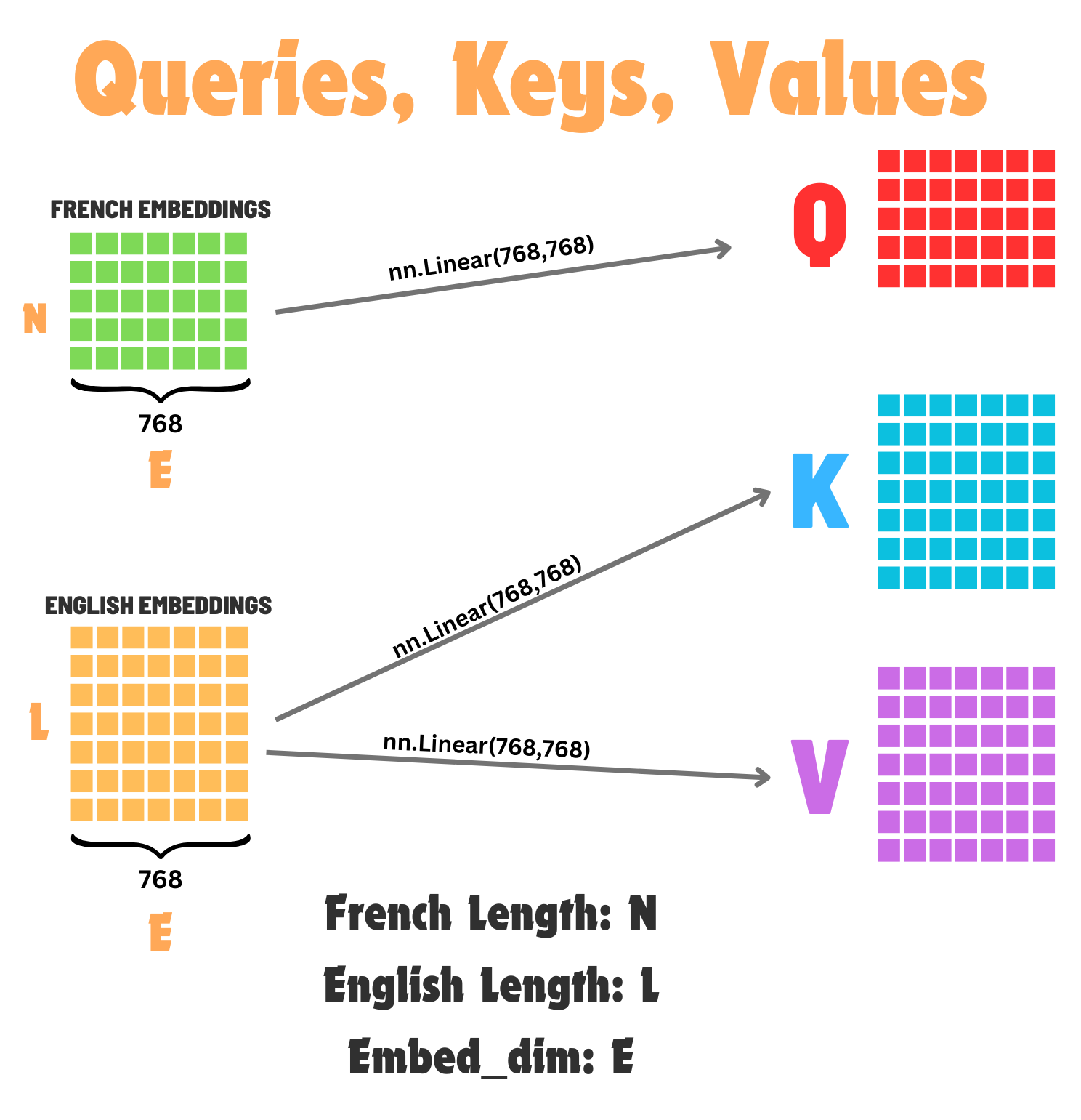
Lets pretend we have an input of French embeddings with \(N\) tokens (with an embedding dimension of \(E\)) and then also English Embeddings with \(L\) tokens (again with an embedding dimension of \(E\)). Again, because the French is what we want, we will project our French embeddings to be our Queries, and then our English Embeddings to our Keys/Values.
French Query Embeddings:
B x N x EEnglish Key Embeddings:
B x L x EEnglish Value Embeddings:
B x L x E
Performing the Attention Computation#
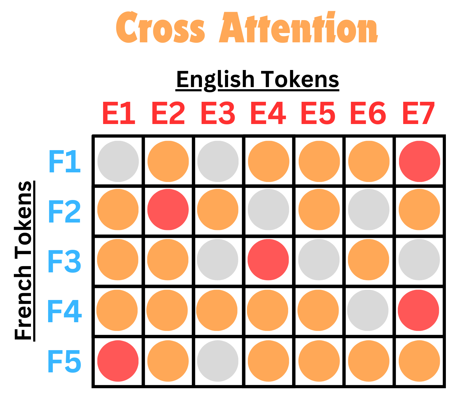
Nothing changes with our attention formula as described. This attention computation is identical to earlier, its just because our Queries is of length \(N\) and the Keys are of length \(L\), our final attention matrix will be an (B x N x L) matrix.
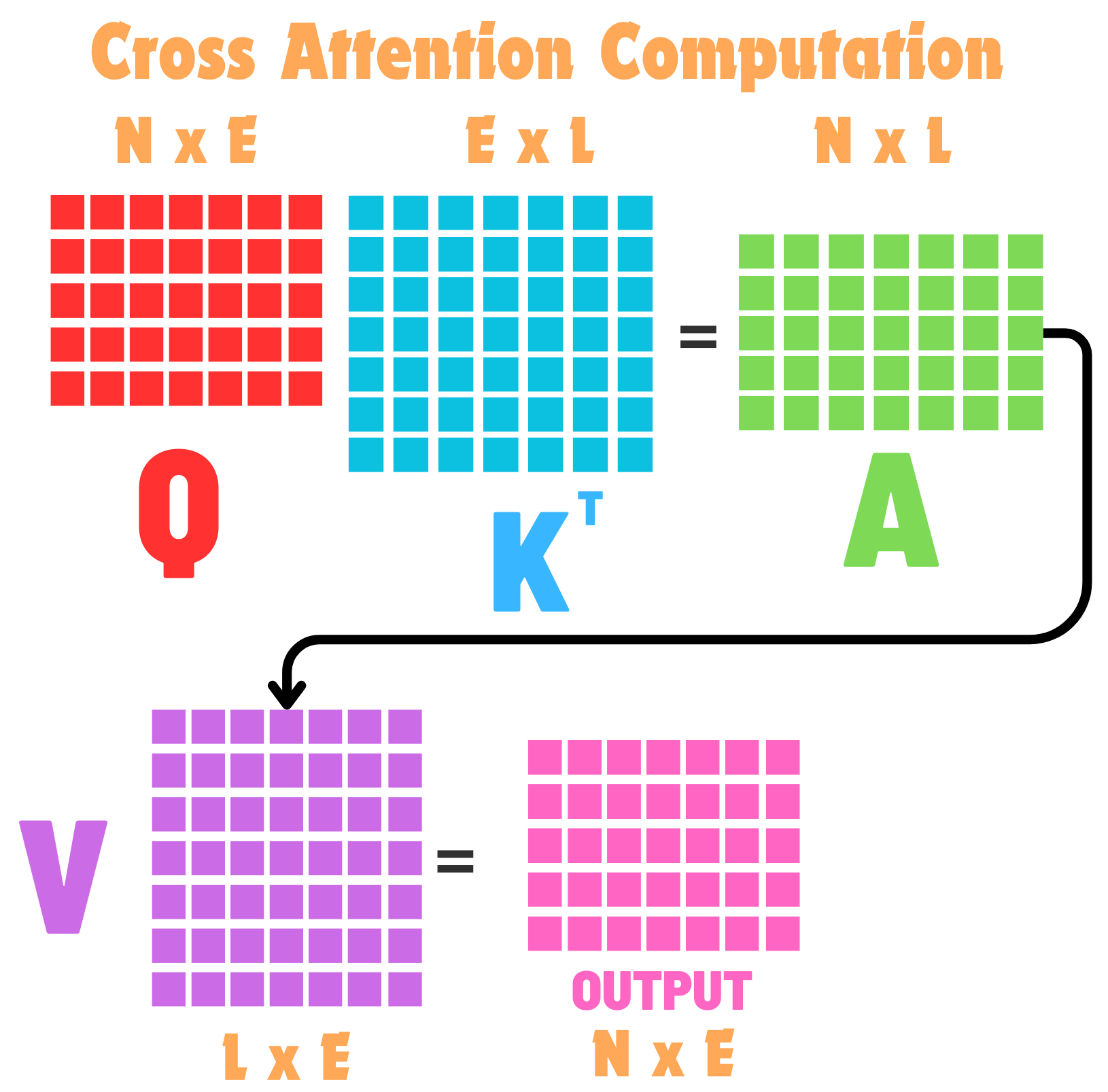
We can take a closer look at our attention matrix now as well, and we see that it isn’t a square matrix anymore, but it still does the same thing: How are each French token related to each English token?
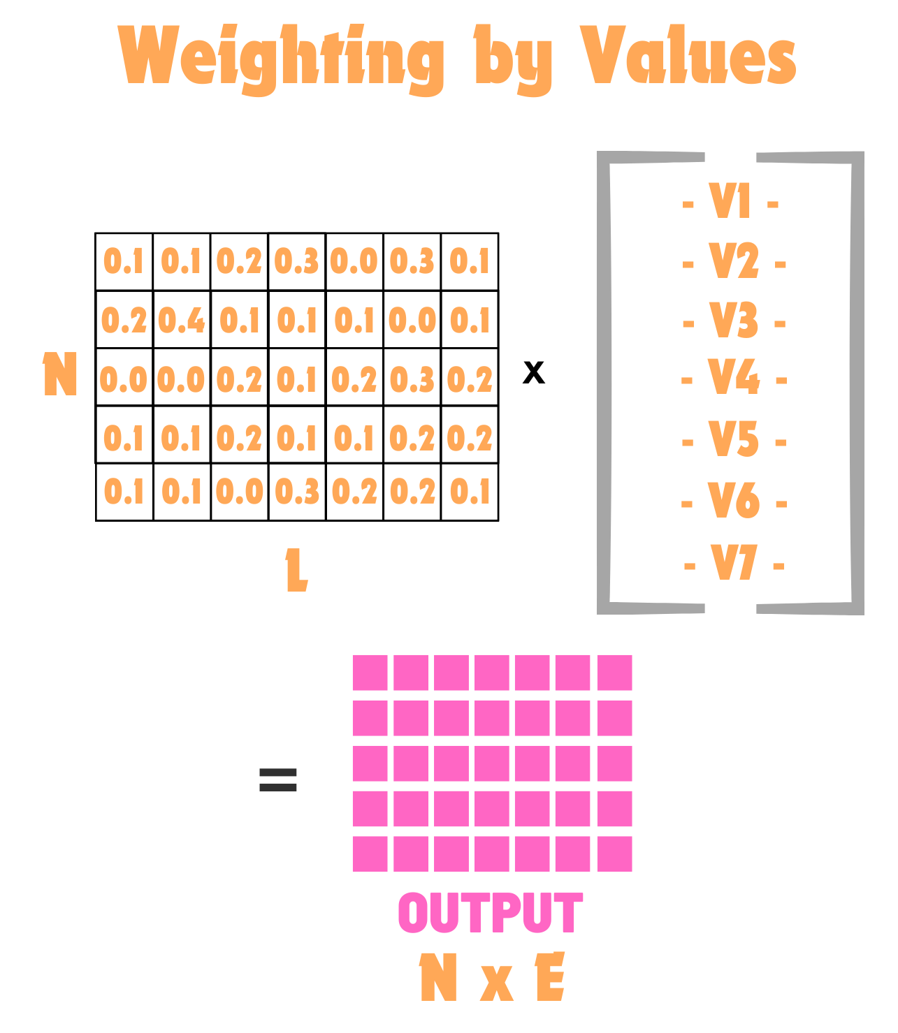
THE MOST IMPORTANT PART!!!#
Once our attention matrix B x N x L is computed, we can again multiply it by our Values matrix which is also from our English embeddings, so we are multiplying a B x N x L by a B x L x E, producing the final output of B x N x E! Why does this matter? Because our original French was also B x N x E! Remember, our attention computation told us how every French token is related to every English token. Then, the output of our full attention computation does the weighted average, so our new B x N x E is the weighted average of those english tokens. Lets see what that looks like:
Basically Nothing Changed#
Nothing really changed in the end! Cross Attention is just attention between two different sequences rather than than one sequence to itself. This means we also have multihead attention (although I didn’t draw it), so nothing changes at all. Cross Attention is ALWAYS an encoder, not autoregressive. It doesnt make sense to have a causal mask here because one sequence can look at the entirety of the other (i.e. our input english can look at all of the generated french). But there is one more caveat:
Padding on English and French#
We are now training a language translation model, this means that when we batch data, both english and french can be padded, and they can be differently padded. For example lets say we have the following data (pairs of english and french tokens)
English: [a1, a2, a3, a4], French: [b1, b2, b3, b4, b5]
English: [c1, c2, c3], French: [d1, d2]
This means, when we batch the english we have to pad the sequence of length 3 to the sequence of length 4.
[a1, a2, a3, a4]
[c1, c2, c3, <PAD>]
And similarly, when we batch the french, we have to pad the sequence of length 2 to the sequence of length 5.
[b1, b2, b3, b4, b5]
[d1, d2, <PAD>, <PAD>, <PAD>]
So we have padding on both dimensions, but again nothing changes. Remember before (in self attention), when we have pad tokens we just zeroed out the columns of the cooresponding pad tokens. But really, we are zeroing out the Keys columns. We want to make sure that when we learn how the French is related to the English, that the French is not looking at English Pad Tokens. It is ok though for French pad tokens to look at English. (i.e. the Query pad tokens can look at the keys, but the Query non-pad tokens should not look at the Key pad tokens). This is what this would again look like:
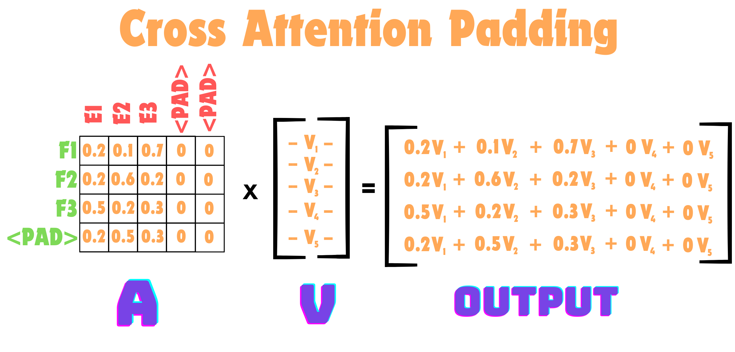
As we can see here, all French tokens (french padding included) can look at all non-padding english tokens. This is identical to what we did before, its just now our attention matrix just isn’t square.
Implementing Cross Attention#
Implementing Cross Attention shouldn’t be all that different from before. There is no causality here, so we only have to keep an eye on the attention mask. We will have two attention masks now, one for the english and another for the french. But when doing English to French Translation, we really just care about the English padding mask, so we can remove those columns from our attention computation. We do need the French padding mask though when we are doing french self-attention, but lets focus on the Cross Attention now
In this implementation, we will be passing in both a src (our English) and tgt (our French).
Matching Shapes for MultiHead Attention#
We again have our attention mask and need to do the reshapes and repeats to get it to the shape necessary to mask our attention computation! Lets take a look at our shapes for Cross Attention again.
attn.shape - (Batch x num_heads x french_seq_len x english_seq_len)
mask.shape - (Batch x english_seq_len)
So just like before, we can take our mask, and add dimensions from Batch x english_seq_len to Batch x 1 x 1 x english_seq_len which would be enough, except our Flash Attention implementation will expect a Batch x 1 x french_seq_len x english_seq_len. So then we can take our Batch x 1 x 1 x english_seq_len and repeat the dummy 1 dimension which is a placeholder for the french_seq_len and repeat it french_seq_len times.
class CrossAttention(nn.Module):
    """
    Cross Attention Proposed in `Attention is All  You Need` - https://arxiv.org/abs/1706.03762
    """

    def __init__(self,
               embed_dim=768,
               num_heads=12,
               attn_p=0,
               proj_p=0):
        """

        Args:
            embed_dim: Transformer Embedding Dimension
            num_heads: Number of heads of computation for Attention
            attn_p: Probability for Dropout2d on Attention cube
            proj_p: Probability for Dropout on final Projection
        """

        super(CrossAttention, self).__init__()

        ### Make Sure Embed Dim is Divisible by Num Heads ###
        assert embed_dim % num_heads == 0
        self.num_heads = num_heads
        self.head_dim = int(embed_dim / num_heads)

        ### Define all our Projections ###
        self.q_proj = nn.Linear(embed_dim, embed_dim)
        self.k_proj = nn.Linear(embed_dim, embed_dim)
        self.v_proj = nn.Linear(embed_dim, embed_dim)
        self.attn_drop = nn.Dropout(attn_p)

        ### Define Post Attention Projection ###
        self.proj = nn.Linear(embed_dim, embed_dim)
        self.proj_drop = nn.Dropout(proj_p)

    def forward(self, src, tgt, attention_mask=None):

        batch, src_seq_len, embed_dim = src.shape
        batch, tgt_seq_len, embed_dim = tgt.shape

        ### Compute Q (on our tgt French) ###
        q = self.q_proj(tgt).reshape(batch, tgt_seq_len, self.num_heads, self.head_dim).transpose(1,2).contiguous()

        ### Compute K, V (on src English) Projections ###
        k = self.k_proj(src).reshape(batch, src_seq_len, self.num_heads, self.head_dim).transpose(1,2).contiguous()
        v = self.v_proj(src).reshape(batch, src_seq_len, self.num_heads, self.head_dim).transpose(1,2).contiguous()

        ### Perform Attention Computation ###
        attn = (q @ k.transpose(-2,-1)) * (self.head_dim ** -0.5)

        ####################################################################################
        ### FILL ATTENTION MASK WITH -Infinity ###

        ### NOTE:
        ### attn.shape - (Batch x num_heads x french_seq_len x english_seq_len)
        ### mask.shape - (Batch x english_seq_len)

        ### Need to expand mask (Batch x english_seq_len) -> (Batch x 1 x 1 x english_seq_len) -> (Batch x 1 x french_seq_len x english_seq_len)

        if attention_mask is not None:
            attention_mask = attention_mask.unsqueeze(1).unsqueeze(1).repeat(1,1,tgt_seq_len,1)
            attn = attn.masked_fill(~attention_mask, float('-inf'))

        ####################################################################################

        attn = attn.softmax(dim=-1)
        attn = self.attn_drop(attn)
        x = attn @ v

        ### Bring Back to [Batch x Seq Len x Embed Dim] ###
        x = x.transpose(1,2).reshape(batch, tgt_seq_len, embed_dim)

        ### Pass through Projection so Heads get to know each other ###
        x = self.proj(x)
        x = self.proj_drop(x)

        return x


### We will now have sequences of different lengths, identify the number of tokens in each sequence ###
english_seq_lens = [3,5,4]
french_seq_lens = [7,6,2]

embed_dim = 18
num_heads = 3
a = CrossAttention(embed_dim, num_heads)

### Create random tensor in the shape (Batch x Seq Len x Embed Dim) for French and English ###
### This will be a tensor upto the max(seq_lens) ###
rand_english = torch.randn(len(english_seq_lens),max(english_seq_lens),embed_dim)
rand_french = torch.randn(len(french_seq_lens),max(french_seq_lens),embed_dim)


### Create Attention Mask from the seq_lens (shortest sequences padded to the longest ###
english_masks = torch.nn.utils.rnn.pad_sequence([torch.ones(l) for l in english_seq_lens], batch_first=True, padding_value=0).bool()
french_masks = torch.nn.utils.rnn.pad_sequence([torch.ones(l) for l in french_seq_lens], batch_first=True, padding_value=0).bool()

print("English Attention Mask:")
print(english_masks)
print("French Attention Mask:")
print(french_masks)

### Pass through MHA ###
output = a(src=rand_english, tgt=rand_french, attention_mask=english_masks)
print("Final Output:", output.shape)
English Attention Mask:
tensor([[ True,  True,  True, False, False],
        [ True,  True,  True,  True,  True],
        [ True,  True,  True,  True, False]])
French Attention Mask:
tensor([[ True,  True,  True,  True,  True,  True,  True],
        [ True,  True,  True,  True,  True,  True, False],
        [ True,  True, False, False, False, False, False]])
Final Output: torch.Size([3, 7, 18])
Flash Attention#
Although our attention computations that we have done are completely correct, they are not the most efficient! Flash Attention is a highly optimized hardware aware attention implementation. For a deep dive into Flash Attention, see this blog post.
Due to the structure of the attention computation you can actually opt for a faster tiled matrix multiplication that fuses the matrix multiplication, softmax and scaling into a single CUDA kernel. We were obviously doing this as separate steps, beacause we don’t have that level of control in PyTorch over CUDA. The most expensive part of GPU operations is copying between global memory and GPU shared memory, and so by merging a bunch of operations together, we just get faster attention computations especially for long sequences.
There are a few places we can access this, but the easiest for us is to use torch.scaled_dot_product_attention (documentation)
This method allows us to pass in:
Queries: (B x H x L x E)Keys: (B x H x S x E)Values: (B x H x S x E)attn_mask: (B x 1 x L x S)
So as you can see, Flash Attention supports our Queries being different from Keys/Values as we saw in our Cross Attention implementation. In the case of self-attention \(L = S\) which also isn’t a problem. The only extra step on our end is to make sure our attn_mask is of shape (B x 1 x L x S), which means we have to do the extra repeat, as it wont automatically broadcast along the \(L\) dimension if we left it as (B x 1 x 1 x S). Flash Attention also expects tokens we don’t want to compute attention on to be False in the attention mask!
The other option that is important it:
is_causal: True/False Boolean indicating if we want a causal mask. The method will apply the causal mask itself so we don’t need to do it!
Lets Add Flash Attention to our Self Attention#
class SelfAttention(nn.Module):
    """
    Self Attention Proposed in `Attention is All  You Need` - https://arxiv.org/abs/1706.03762
    """

    def __init__(self,
                 embed_dim=768,
                 num_heads=12,
                 attn_p=0,
                 proj_p=0,
                 causal=False,
                 fused_attn=True):
        """

        Args:
            embed_dim: Transformer Embedding Dimension
            num_heads: Number of heads of computation for Attention
            attn_p: Probability for Dropout2d on Attention cube
            proj_p: Probability for Dropout on final Projection
            causal: Do you want to apply a causal mask?
        """

        super(SelfAttention, self).__init__()

        ### Make Sure Embed Dim is Divisible by Num Heads ###
        assert embed_dim % num_heads == 0
        self.num_heads = num_heads
        self.head_dim = int(embed_dim / num_heads)
        self.causal = causal
        self.fused = fused_attn

        ### Define all our Projections ###
        self.q_proj = nn.Linear(embed_dim, embed_dim)
        self.k_proj = nn.Linear(embed_dim, embed_dim)
        self.v_proj = nn.Linear(embed_dim, embed_dim)
        self.attn_drop = nn.Dropout(attn_p)

        ### Define Post Attention Projection ###
        self.proj = nn.Linear(embed_dim, embed_dim)
        self.proj_drop = nn.Dropout(proj_p)

    def forward(self, x, attention_mask=None):

        batch, seq_len, embed_dim = x.shape

        ### Compute Q, K, V Projections,and Reshape/Permute to [Batch x Num Heads x Seq Len x Head Dim]
        q = self.q_proj(x).reshape(batch, seq_len, self.num_heads, self.head_dim).transpose(1,2).contiguous()
        k = self.k_proj(x).reshape(batch, seq_len, self.num_heads, self.head_dim).transpose(1,2).contiguous()
        v = self.v_proj(x).reshape(batch, seq_len, self.num_heads, self.head_dim).transpose(1,2).contiguous()

        ### Use Flash Attention ###
        if self.fused:

            x = F.scaled_dot_product_attention(q,k,v,
                                               is_causal=self.causal,
                                               attn_mask=attention_mask)

        else:

            ### Perform Attention Computation ###
            attn = (q @ k.transpose(-2,-1)) * (self.head_dim ** -0.5)


            if self.causal:
                ####################################################################################
                ### Create the Causal Mask (On the correct device) ###

                ### Create a Seq_Len x Seq_Len tensor full of Ones
                ones = torch.ones((seq_len, seq_len), device=attn.device)

                ### Fill Top right triangle with Zeros (as we dont want to attend to them) ###
                causal_mask = torch.tril(ones)

                ### Add extra dimensions for Batch size and Number of Heads ###
                causal_mask = causal_mask.reshape(1,1,seq_len,seq_len).bool()

                ### If we have padding mask, then update our causal mask ###
                if attention_mask is not None:

                    ### Each sample could have a different number of pad tokens, so repeat causal mask for batch size ###
                    causal_mask = causal_mask.repeat(batch, 1, 1, 1)

                    ### Expand and repeat the Padding Mask (b x s) -> (b x 1 x s x s)###
                    attention_mask = attention_mask.unsqueeze(1).unsqueeze(1).repeat(1,1,seq_len,1)

                    ### Fill causal mask where attention mask is False with False (to ensure all padding tokens are masked out) ###
                    causal_mask = causal_mask.masked_fill(~attention_mask, False)

                ### Fill attn with -inf wherever causal mask is False ###
                attn = attn.masked_fill(~causal_mask, float('-inf'))

            ####################################################################################

            attn = attn.softmax(dim=-1)
            attn = self.attn_drop(attn)
            x = attn @ v

        ### Bring Back to [Batch x Seq Len x Embed Dim] ###
        x = x.transpose(1,2).reshape(batch, seq_len, embed_dim)

        ### Pass through Projection so Heads get to know each other ###
        x = self.proj(x)
        x = self.proj_drop(x)

        return x
Putting it All Together#
Obviously, we would like to use Flash Attention for Everything, but we have a few moving pieces right now:
We can have self-attention on a source with padding mask
We can have self-attention on a source with padding mask and causal mask
We can have cross attention between a source and target
Lets write our final Attention computation, putting all of these things together. Again, lets set the stage in terms of and English (src) to French (tgt) translation:
Attention Class Details#
This class will handle all the cases we need. Lets pretend we are doing English to French
We can provide English as the src along with its padding mask for Encoder self-attention
We can provide French as the src along with its padding mask and causal as True for decoder self-attention
We can provide English as src and French as tgt along with the src padding_mask for cross attention
All of this should be very familiar now as we have implemented all the pieces of this already! Its just time to put it together!
Attention Mask for Self-Attention#
Attention Mask is in Batch x Sequence Length where we have False for tokens we don’t want to attend to. F.scaled_dot_product_attention expects a mask of the shape Batch x ..., x Seq_len x Seq_len, where the “…” in this case is any extra dimensions (such as heads of attention). Lets expand our mask to Batch x 1 x Seq_len x Seq_len. The 1 in this case refers to the number of heads of attention we want, so it is a dummy index to broadcast over. In each Seq_len x Seq_len matrix for every batch, we want False for all columns corresponding to padding tokens.
Attention Mask for Cross-Attention#
When doing cross attention, our French will be Batch x french_len x embed_dim and our English will be Batch x english_len x embed_dim. In typical cross attention fashion, the queries will be the thing we want and Keys/Values will be the thing we are crossing with. In our Decoder Cross Attention, we want to learn how our generated French is related to the encoded english from the Encoder. So our Queries will be French and Keys/Values will be the encoded English.
\(Q\) @ \(K^T\) will then give a shape Batch x ... x french_len x english_len. This means our attention mask also has to have this shape. Just like before, we want to mask out the columns of the attention mask, so our french tokens dont attend to any english padding tokens. We can then take our english padding mask which is (Batch x english_len), add extra dimensions for head and src_len dimension which will give a Batch x 1 x 1 x english_len and then repeat the mask for the source length batch x 1 x french_len x english_len.
class Attention(nn.Module):
    """
    Regular Self-Attention but in this case we utilize flash_attention
    incorporated in the F.scaled_dot_product_attention to speed up our training.
    """
    def __init__(self, embedding_dimension=768, num_heads=12, attn_dropout=0.0):
        super(Attention, self).__init__()

        self.embedding_dimension = embedding_dimension
        self.num_heads = num_heads
        self.attn_dropout = attn_dropout

        ### Sanity Checks ###
        assert embedding_dimension % num_heads == 0, "Double check embedding dim divisible by number of heads"

        ### Attention Head Dim ###
        self.head_dim = embedding_dimension // num_heads

        ### Attention Projections ###
        self.q_proj = nn.Linear(embedding_dimension, embedding_dimension)
        self.k_proj = nn.Linear(embedding_dimension, embedding_dimension)
        self.v_proj = nn.Linear(embedding_dimension, embedding_dimension)

        ### Post Attention Projection ###
        self.out_proj = nn.Linear(embedding_dimension, embedding_dimension)


    def forward(self,
                src,
                tgt=None,
                attention_mask=None,
                causal=False):

        """
        By default, self-attention will be computed on src (with optional causal and/or attention mask). If tgt is provided, then
        we are doing cross attention. In cross attention, an attention_mask can be used, but no causal mask can be applied.
        """

        ### Grab Shapes ###
        batch, src_len, embed_dim = src.shape

        ### If target is not provided, we are doing self attention (with potential causal mask) ###
        if tgt is None:
            q = self.q_proj(src).reshape(batch, src_len, self.num_heads, self.head_dim).transpose(1,2).contiguous()
            k = self.k_proj(src).reshape(batch, src_len, self.num_heads, self.head_dim).transpose(1,2).contiguous()
            v = self.v_proj(src).reshape(batch, src_len, self.num_heads, self.head_dim).transpose(1,2).contiguous()

            if attention_mask is not None:

                attention_mask = attention_mask.bool()
                attention_mask = attention_mask.unsqueeze(1).unsqueeze(1).repeat(1,1,src_len,1)

            attention_out = F.scaled_dot_product_attention(q,k,v,
                                                           attn_mask=attention_mask,
                                                           dropout_p=self.attn_dropout if self.training else 0.0,
                                                           is_causal=causal)

        ### If target is provided then we are doing cross attention ###
        ### Our query will be the target and we will be crossing it with the encoder source (keys and values) ###
        ### The src_attention_mask will still be the mask here, just repeated to the target size ###
        else:
            tgt_len = tgt.shape[1]

            q = self.q_proj(tgt).reshape(batch, tgt_len, self.num_heads, self.head_dim).transpose(1,2).contiguous()
            k = self.k_proj(src).reshape(batch, src_len, self.num_heads, self.head_dim).transpose(1,2).contiguous()
            v = self.v_proj(src).reshape(batch, src_len, self.num_heads, self.head_dim).transpose(1,2).contiguous()

            if attention_mask is not None:

                attention_mask = attention_mask.bool()
                attention_mask = attention_mask.unsqueeze(1).unsqueeze(1).repeat(1,1,tgt_len,1)

            attention_out = F.scaled_dot_product_attention(q,k,v,
                                                           attn_mask=attention_mask,
                                                           dropout_p=self.attn_dropout if self.training else 0.0,
                                                           is_causal=False)

        ### Reshape and Project ###
        attention_out = attention_out.transpose(1,2).flatten(2)
        attention_out = self.out_proj(attention_out)

        return attention_out

### Test Out Self-Attention!! ###
print("TESTING SELF-ATTENTION!!!")
print("-------------------------")
seq_lens = [3,5,4]
embed_dim = 9
num_heads = 3
a = Attention(embed_dim, num_heads)

### Create a random tensor in the shape (Batch x Seq Len x Embed Dim) ###
### This will be a tensor upto the max(seq_lens) ###
rand = torch.randn(len(seq_lens),max(seq_lens),embed_dim)

### Create Attention Mask from the seq_lens (shortest sequences padded to the longest ###
masks = torch.nn.utils.rnn.pad_sequence([torch.ones(l) for l in seq_lens], batch_first=True, padding_value=0).bool()
print("Attention Mask:")
print(masks)

### Pass through MHA ###
output = a(rand, attention_mask=masks, causal=False) # causal=false to remove an error setting with mask
print("Final Output:", output.shape, "\n")


print("TESTING CROSS-ATTENTION!!!")
print("-------------------------")
### Test out Cross Attention
### We will now have sequences of different lengths, identify the number of tokens in each sequence ###
english_seq_lens = [3,5,4]
french_seq_lens = [7,6,2]

embed_dim = 9
num_heads = 3
a = Attention(embed_dim, num_heads)

### Create random tensor in the shape (Batch x Seq Len x Embed Dim) for French and English ###
### This will be a tensor upto the max(seq_lens) ###
rand_english = torch.randn(len(english_seq_lens),max(english_seq_lens),embed_dim)
rand_french = torch.randn(len(french_seq_lens),max(french_seq_lens),embed_dim)


### Create Attention Mask from the seq_lens (shortest sequences padded to the longest ###
english_masks = torch.nn.utils.rnn.pad_sequence([torch.ones(l) for l in english_seq_lens], batch_first=True, padding_value=0).bool()
french_masks = torch.nn.utils.rnn.pad_sequence([torch.ones(l) for l in french_seq_lens], batch_first=True, padding_value=0).bool()

print("English Attention Mask:")
print(english_masks)
print("French Attention Mask:")
print(french_masks)

### Pass through MHA ###
output = a(src=rand_english, tgt=rand_french, attention_mask=english_masks)
print("Final Output:", output.shape)
TESTING SELF-ATTENTION!!!
-------------------------
Attention Mask:
tensor([[ True,  True,  True, False, False],
        [ True,  True,  True,  True,  True],
        [ True,  True,  True,  True, False]])
Final Output: torch.Size([3, 5, 9])

TESTING CROSS-ATTENTION!!!
-------------------------
English Attention Mask:
tensor([[ True,  True,  True, False, False],
        [ True,  True,  True,  True,  True],
        [ True,  True,  True,  True, False]])
French Attention Mask:
tensor([[ True,  True,  True,  True,  True,  True,  True],
        [ True,  True,  True,  True,  True,  True, False],
        [ True,  True, False, False, False, False, False]])
Final Output: torch.Size([3, 7, 9])
Thats It!#
That is basically everything you need to know about attention! Now if you are actually going to be using attention in your model, it is better to use optimized CUDA implementations rather than this only for speed and efficiency reasons, but they are doing exactly the same thing underneath the hood, just faster! This sets us up though for the next step! All we have done so far is implement the Attention mechanism, this is only half the picture for the Transformer. There are bunch of directions one can now go:
Seq2Seq Models (Language Translation, Image Captioning)
Encoder Models (RoBERTa, Vision Transformer)
Decoder Models (GPT, LLAMA)
Acknowledgments#
Initial version: Mark Neubauer
Modified from the following Tutorial
© Copyright 2026