Beam Angle Optimization for Radiative Cancer Therapy

Beam Angle Optimization for Radiative Cancer Therapy#

Overview#

In November 1895, Wilhelm Röntgen accidentally discovered X-rays while fiddling with cathode ray tubes. He proceeded to pass these rays through his wife’s hand to create the world’s first X-ray image. This was a pivotal time for the field of medical physics (and their marriage): a means to harness physics phenomena to better the human condition.

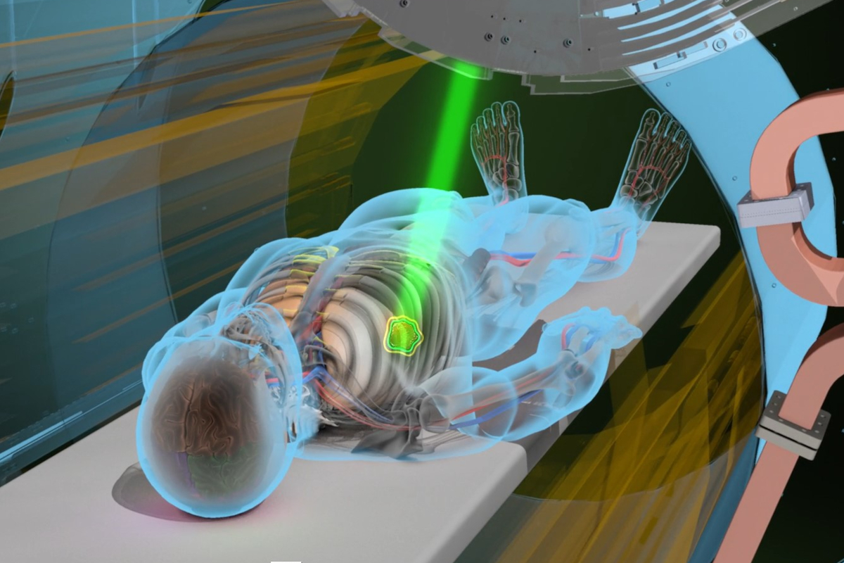
Today, radiation therapy involves firing intense beams of ionizing radiation to obliterate cancer cell DNA and halt the malicious growth of tumors. A patient is often laid before a gantry, essentially a LINAC accelerator, that ejects X-rays (or protons, when further precision is required). A rigorous treatment plan requires consideration of:

The ‘dose’ of radiation that a patient can handle (determined by understanding the physical interactions of radiation with tissue)
Beam-Angle Optimization (BAO): annihilating cancerous tissue while preserving healthy cells. BAO involves finding the ideal set of beam paths to accomplish precisely this goal. The machine learning methods we’ve studied thus far have been instrumental in better resolving this combinatorial problem

We will be extracting patient head-neck CT scan + mask data (our ‘input’) from the medical physics OpenKBP challenge. This is real clinical data, and you could make significant contributions to healthcare and cancer treatment by going above & beyond what you learn here!

Data Sources#

Original Source

ababier/open-kbp

Local Copy URL

https://courses.physics.illinois.edu/phys498mlp/sp2025/data/projects/RadioTherapy/openkbp_patient_data.zip

Questions#

Question 01: Absorption & Scattering#

X-rays attenuate exponentially upon entering the body by the Beer-Lambert Law.

\[ I(x) = I_0 e^{-\mu x} \]

\[\begin{split} \begin{aligned} x & : \text{Depth in the body} \\ I(x) & : \text{Intensity at depth } x \\ I_0 & : \text{Initial intensity (at the skin)} \\ \mu & : \text{Linear attenuation coefficient (depends on whether we traverse bone, soft tissue or organs) } \end{aligned} \end{split}\]

What physical phenomena govern this loss of intensity (state at least 3 specific processes)? Which one dominates radiotherapy (which uses ~6 MeV photons)? It’s easy to conclude that the highest dose of radiation is delivered at the skin, why is this untrue?

Question 02: Dosimetry#

We quantify the impact of radiation on tissue (be it healthy or cancerous) via a metric known as Dose. It is the ratio between the energy absorbed and the mass of the tissue absorbing it: measured in Gray (Gy).

\[ \text{Dose} = \frac{dE}{dm} \quad \text{where} \quad dE = \text{energy deposited (Joules)}, \quad dm = \text{mass of tissue (kilograms)} \]

What are the implications of too little or too much Dose? Does the type of body tissue matter? Putting it all together, what are the factors which determine the ideal beam angles a gantry should use? For instance, what are the risks to patient health? Why do these considerations make Beam Angle Optimization (BAO) an NP-hard problem?

Question 03: Proton Therapy#

If we used proton therapy instead of X-rays, how would our considerations evolve?

Question 04: Preparing Tensors#

Run the cell below and unzip the contents of openkbp_patient_data into a folder. It should be present in Colab’s (/content/..) or local directory. Note that you will need to adjust base_path to lead to this folder.

Each patient hosts the following three files:
ct.csv - 3D grayscale CT scan of patient anatomy composed of 2D slices. Each voxel represents how much X-ray is absorbed by the tissue in Hounsfield Units (HU)
PTV63.csv - Planning Target Volume (PTV) is a sparse mask that maps the location of the tumor. We’d like binary mask so that 1 is tumor, 0 is no-tumor.

The following are sparse masks of Organs at Risk (OAR), representing what we’d like our beams to avoid

SpinalCord.csv - Irradiating the spine can cause a serious condition known as radiation myelopathy.
Brainstem.csv - Radiation causes a vast myriad of devastating effects like RIBN, Ataxia, or even comas.
LeftParotid.csv, RightParotid.csv - Irradiating salivary glands can cause xerostomia (dry mouth) or worse
Mandible.csv - The mandible has a limited blood supply, and osteoradionecrosis can occur YEARS after treatment.

These are flattened volumes with voxel indices. The cell below converts the csv files into binary 3D volumes [128, 128, 128] where each point represents an intensity (for the ct scan) or binary value (for ptv & spinal cord). You will have an optional dictionary of patient_data to access for your convenience.

Your tasks:

Add a line to the for loop that stacks ct, ptv, and oars (Organs at Risk) into a single tensor. Note that oars is a dictionary you may need to unpack. What’s the final shape of this tensor? Draw an analogy to an RGB image.
Visualize a single 2D axial slice (z-axis slice) of a patient’s CT scan with the tumor(ptv) overlaid…as a sanity check.

!wget https://github.com/florilegium7/Physics-informed-DQN-Radiotherapy/releases/download/v1/openkbp_patient_data.zip
!unzip openkbp_patient_data.zip -d openkbp_patient_data

import numpy as np
import pandas as pd
import os

base_path = 'openkbp_patient_data' #you may adjust this (e.g. /content/openkbp_patient_data)

patient_ids = ["pt_1", "pt_2", "pt_9","pt_40","pt_68","pt_70", "pt_90", "pt_91" , "pt_99", "pt_187"]
patient_tensors = []

def mask_from_sparse(path,shape=(128, 128,128)): #converts voxel indices to 3D binary masks!
    indices = pd.read_csv(path, header=None)[0].dropna().astype(int).values
    mask_flat = np.zeros(np.prod(shape), dtype=np.uint8)
    mask_flat[indices] = 1
    return mask_flat.reshape(shape)

def sparse_to_ct_volume(path, shape=(128, 128, 128)): #turns the csv into full 3D volume CT scans
    df = pd.read_csv(path, header=None).dropna()
    indices = df[0].astype(int).values
    values = df[1].astype(float).values
    ct_flat = np.zeros(np.prod(shape), dtype=np.float32)
    ct_flat[indices] = values
    return ct_flat.reshape(shape)


#128 x 128 x 128 pixels : (depth, height, width)
for pt_id in patient_ids:

    pt_dir = os.path.join(base_path, pt_id)

    ct = sparse_to_ct_volume(os.path.join(pt_dir, "ct.csv"))
    ptv = mask_from_sparse(os.path.join(pt_dir, "PTV63.csv"))

    oars = {} #dictionary
    organs = ["SpinalCord", "Brainstem", "LeftParotid", "RightParotid", "Mandible"]
    for organ in organs:
        organ_path = os.path.join(pt_dir, f"{organ}.csv")
        if os.path.exists(organ_path):
            oars[organ] = mask_from_sparse(organ_path)
    
    patient_data = {
        "id": pt_id,
        "ct": ct, #ct scan -> 3D volume with intensities
        "ptv": ptv, #tumor -> 3D binary mask (1 means tumor!)
        "oars": oars #dictionary of organs at risk -> each is a 3D binary mask
    }
    

    pt_tensor = #Your Code Here 
    patient_tensors.append(pt_tensor)

#Your slice visualization here
import matplotlib.pyplot as plt

Question 05: Reinforcement Learning#

To simulate the effects of a naive beam (simple straight lines) passing through the patient, we provide a ‘beam mask’ that creates a beam onto a 2D slice of the patient scan. We assume there are 36 possible angles from which a beam can be fired (one every 10 degrees). dose is a 2D heatmap that represents how much radiation is delivered to each pixel in your slice after the passage of many beams.

Create a Reinforcement Learning Model which selects beam angles that provide radiation dosage to the tumor while avoiding the spinal cord.

Populate the training loop by:
- Creating a policy that determines the next angle
- Creating a Q-learning update
Define a reward function that heavily penalizes a beam that passes through the spinal cord and rewards a beam that hits the tumor/ptv (the output should be a score)
Tweak parameters if you so desire
Print the top 3 beam angles after training is complete

import random

beam_angles = np.arange(0, 360, 10)  #[0, 10, 20, ..., 350]
max_beams = 5 #ensures beams are chosen strategically
episodes = 500
alpha = 0.1 #learning rate
epsilon = 0.2 #exploration rate
slice_shape = (128,128) #a single 2D slice

from skimage.draw import line_nd

def generate_beam(angle_deg, shape): #beam mask generator! 
    h, w = shape
    beam_mask = np.zeros((h, w), dtype=np.uint8)
    center = np.array([h // 2, w // 2])
    length = max(h, w)
    angle_rad = np.deg2rad(angle_deg)

    dx = np.cos(angle_rad)
    dy = np.sin(angle_rad)
    start = (center - length * np.array([dy, dx])).astype(int)
    end   = (center + length * np.array([dy, dx])).astype(int)
    start = np.clip(start, 0, [h - 1, w - 1])
    end   = np.clip(end,   0, [h - 1, w - 1])
    rr, cc = line_nd(start[0], start[1], end[0], end[1])
    beam_mask[rr, cc] = 1
    return beam_mask


for episode in range(episodes):
    #Randomly select a patient from patient_tensors HERE

    #extracts a single 2D slice from the middle
    mid = ct.shape[2] // 2 
    ct_slice   = ct[:, :, mid]
    ptv_slice  = ptv[:, :, mid]
    #extract organ slices HERE

    dose = np.zeros(slice_shape, dtype=np.float32)
    selected_angles = []

    for i in range(max_beams):
        #Your policy here

        beam = generate_beam(angle, slice_shape)
        dose += beam.astype(np.float32) #adds 'radiation' to the pixels 
        selected_angles.append(angle)

    
    reward_score = reward(dose, ptv, organs)

    for angle in selected_angles:
        #Q-learning update here



def reward(dose, ptv, organs): #your reward function HERE
    raise NotImplementedError()
 

Q = np.zeros(len(beam_angles)) #Q-table

Your model (have you named it yet?) has chosen its ideal beam angles, let’s cross our fingers, fire these into our patient, and see what we get!

import matplotlib as plt


patient = random.choice(patient_tensors)
mid = patient.shape[3] // 2
ct, ptv, cord = patient[0, :, :, mid], patient[1, :, :, mid], patient[2, :, :, mid]
shape = ct.shape
dose = np.zeros(shape, dtype=np.float32)
top_indices = sorted(range(len(Q)), key=lambda i: -Q[i])[:max_beams]
selected_angles = [beam_angles[i] for i in top_indices]

for angle in selected_angles:
    beam = generate_beam(angle, shape)
    dose += beam.astype(np.float32)

plt.imshow(ct, cmap='gray')
plt.imshow(dose, cmap='hot', alpha=0.4)
plt.contour(ptv, colors='green')
plt.contour(cord, colors='blue')
for angle in selected_angles:
    plt.imshow(generate_beam(angle, shape), cmap='Reds', alpha=0.2)
plt.title(f"Selected Beams: {selected_angles}\nPTV: Green, Cord: Blue")
plt.axis('off')
plt.show()

Question 06: Physics-informed reinforcement learning#

Ready to boogie? We’re about to imbue physics into our RL model. Let’s start by making our beam of ionizing radiaiton more realistic using what we discussed in Question 01. Adjust the decay in generate_true_beam below so that it actually attenuates our beam (energy loss as it passes through tissue)

def generate_physical_beam(angle_deg, shape = (128,128), spread_sigma=2.0, attenuation_coeff=0.01):
    h, w = shape
    beam_mask = np.zeros((h, w), dtype=np.float32)
    center = np.array([h // 2, w // 2])
    length = max(h, w)
    angle_rad = np.deg2rad(angle_deg)

    dx = np.cos(angle_rad)
    dy = np.sin(angle_rad)
    start = (center - length * np.array([dy, dx])).astype(int)
    end   = (center + length * np.array([dy, dx])).astype(int)
    start = np.clip(start, 0, [h - 1, w - 1])
    end   = np.clip(end,   0, [h - 1, w - 1])

    rr, cc = line_nd(start, end)
    rr = np.clip(rr, 0, h-1)
    cc = np.clip(cc, 0, w-1)

    for i, (r, c) in enumerate(zip(rr, cc)):
        decay =  #attenuatation by Beer-Lambert Law
        beam_mask[r, c] += decay

        for dr in range(-3, 4):  #gaussian spread via scattering
            for dc in range(-3, 4):
                r_spread = r + dr
                c_spread = c + dc
                if 0 <= r_spread < h and 0 <= c_spread < w:
                    distance = np.sqrt(dr**2 + dc**2)
                    spread_value = np.exp(- (distance**2) / (2 * spread_sigma**2))
                    beam_mask[r_spread, c_spread] += decay * spread_value 

    beam_mask = np.clip(beam_mask, 0, 1.0)  
    return beam_mask

We’d like to inject a physics loss that encodes the actual attenuation and radiation dose delivery of the beam, rewarding correct dose distribution between the spine and tumor. We need to upgrade our simple Q-learning method into a Deep-Q Network (DQN). This should only require simple structural changes (refer to our reinforcement learning notebook). Typically, these would use a Bellman loss. With our new physics-loss it should resemble: $$ L_{\text{Total}} = L_{\text{Bellman}} + \lambda_{\text{Physics}} L_{\text{Physics}} $$

The physics loss takes the following form: $$ L_{\text{Physics}} = \lambda_{\text{PTV}} \cdot \text{Underdose}_{\text{PTV}} + \lambda_{\text{Spine}} \cdot \text{Overdose}_{\text{Spine}} $$ Each $\lambda$ assigns 'weight' to a term, tinkering with these may prove beneficial. The Underdose term penalizes not giving the tumor the maximum dose (1) $$ \text{Underdose}_{\text{PTV}} = \mathbb{E} \left[ \max \left( 0,\ 1 - D_{\text{PTV}} \right) \right] $$

$D_{\text{PTV}}$: dose received by pixels inside the tumor (PTV mask)
$1 - D_{\text{PTV}}$: underdose per pixel (1 is max dose)
$\max(0, 1 - D_{\text{PTV}})$: penalizes only underdosed regions
$\mathbb{E}[\cdot]$: average

The Overdose term penalizes giving the spine too much dose $$ \text{Overdose}_{\text{Spine}} = \mathbb{E} \left[ \max \left( 0,\ D_{\text{Spine}} - D_{\text{safe}} \right) \right] $$

$D_{\text{safe}}$: Safety threshold for organ (max dose it can receive). In clinical settings, this is often 0.6

Now create that network, like a true ML-infused medical physicist of the 21st century would!

#Your masterpiece here

For our grand finale we will overlay your newfound results onto a CT scan of a tumor. Congratulations! You just made a treatment plan for a cancer patient!!

#your conclusions
selected_angles = 

# Choose a patient!
patient = patient_tensors[0]



ct_volume = patient["ct"]
ptv_volume = patient["ptv"]
spine_volume = patient["spine"]
mid = ct_volume.shape[2] // 2
ct_slice = ct_volume[:, :, mid]
ptv_slice = ptv_volume[:, :, mid]
spine_slice = spine_volume[:, :, mid]


def visualize_beams_on_ct(ct_slice, ptv_slice, spine_slice, selected_angles, shape=(128, 128)):
    dose = np.zeros(shape, dtype=np.float32)
    for angle in selected_angles:
        beam = generate_physical_beam(angle, shape)
        dose += beam.astype(np.float32)
    dose_norm = dose / np.max(dose + 1e-5)
    plt.figure(figsize=(6, 6))
    plt.imshow(ct_slice, cmap='gray', alpha=0.6)
    plt.imshow(dose_norm, cmap='hot', alpha=0.4)  #beam
    plt.contour(ptv_slice, colors='red', linewidths=1, label='PTV')
    plt.contour(spine_slice, colors='blue', linewidths=1, label='Spine')
    plt.title("Treatment Plan")
    plt.axis('off')
    plt.colorbar(label="Relative Beam Intensity")
    plt.show()


visualize_beams_on_ct(ct_slice, ptv_slice, spine_slice, selected_angles)

References#

[1] A. Babier, B. Zhang, R. Mahmood, K.L. Moore, T.G. Purdie, A.L. McNiven, T.C.Y. Chan, “OpenKBP: The open-access knowledge-based planning grand challenge and dataset,” Medical Physics, Vol. 48, pp. 5549-5561, 2021.

Acknowledgements#

Initial version: Aarya Mehta with some guidance from Mark Neubauer