Physics Informed Neural Networks

Introduction

Physics-Informed Neural Networks (PINNs) are a novel class of machine learning algorithms for solution of partial differential equations. This is achieved by incorporating structured prior information derived from physical laws into the learning algorithm. PINNs are constructed by encoding the constraints posed by a given differential equation and its boundary conditions into the loss function of a NN. This constraint guides the network to approximate the solution of the differential equation.

ID Harmonic Oscillator Example

Problem Overview

The example problem we solve here is the 1D damped harmonic oscillator:

\[ \Large m \dfrac{d^2 x}{d t^2} + \mu \dfrac{d x}{d t} + kx = 0~, \]

with the initial conditions

\[ \Large x(0) = 1~~,~~\dfrac{d x}{d t} = 0~. \]

We will focus on solving the problem for the under-damped state, i.e. when

\[ \Large \delta < \omega_0~,~~~~~\mathrm{with}~~\delta = \dfrac{\mu}{2m}~,~\omega_0 = \sqrt{\dfrac{k}{m}}~. \]

This has the following exact solution:

\[ \Large x(t) = e^{-\delta t}(2 A \cos(\phi + \omega t))~,~~~~~\mathrm{with}~~\omega=\sqrt{\omega_0^2 - \delta^2}~. \]

Workflow Overview

First we will train a standard neural network to interpolate a small part of the solution, using some observed training points from the solution.

Next, we will train a PINN to extrapolate the full solution outside of these training points by penalising the underlying differential equation in its loss function.

Enviornment Setup

We train the PINN using PyTorch, using the following environment and helper functions:

from PIL import Image

import numpy as np
import torch
import torch.nn as nn
import matplotlib.pyplot as plt

def save_gif_PIL(outfile, files, fps=5, loop=0):
    "Helper function for saving GIFs"
    imgs = [Image.open(file) for file in files]
    imgs[0].save(fp=outfile, format='GIF', append_images=imgs[1:], save_all=True, duration=int(1000/fps), loop=loop)

def oscillator(d, w0, x):
    """Defines the analytical solution to the 1D underdamped harmonic oscillator problem. 
    Equations taken from: https://beltoforion.de/en/harmonic_oscillator/"""
    assert d < w0
    w = np.sqrt(w0**2-d**2)
    phi = np.arctan(-d/w)
    A = 1/(2*np.cos(phi))
    cos = torch.cos(phi+w*x)
    sin = torch.sin(phi+w*x)
    exp = torch.exp(-d*x)
    y  = exp*2*A*cos
    return y

Define the PINN

class FCN(nn.Module):
    "Defines a connected network"
    
    def __init__(self, N_INPUT, N_OUTPUT, N_HIDDEN, N_LAYERS):
        super().__init__()
        activation = nn.Tanh
        self.fcs = nn.Sequential(*[
                        nn.Linear(N_INPUT, N_HIDDEN),
                        activation()])
        self.fch = nn.Sequential(*[
                        nn.Sequential(*[
                            nn.Linear(N_HIDDEN, N_HIDDEN),
                            activation()]) for _ in range(N_LAYERS-1)])
        self.fce = nn.Linear(N_HIDDEN, N_OUTPUT)
        
    def forward(self, x):
        x = self.fcs(x)
        x = self.fch(x)
        x = self.fce(x)
        return x

Generate the Training Data

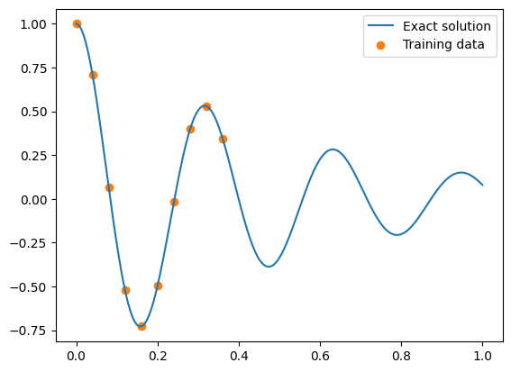
First, we generate some training data from a small part of the true analytical solution.

For this problem, we use \(\delta=2\), \(\omega_0=20\), and try to learn the solution over the domain \(x\in [0,1]\).

d, w0 = 2, 20

# get the analytical solution over the full domain
x = torch.linspace(0,1,500).view(-1,1)
y = oscillator(d, w0, x).view(-1,1)
print(x.shape, y.shape)

# slice out a small number of points from the LHS of the domain
x_data = x[0:200:20]
y_data = y[0:200:20]
print(x_data.shape, y_data.shape)

plt.figure()
plt.plot(x, y, label="Exact solution")
plt.scatter(x_data, y_data, color="tab:orange", label="Training data")
plt.legend()
plt.show()

torch.Size([500, 1]) torch.Size([500, 1])
torch.Size([10, 1]) torch.Size([10, 1])

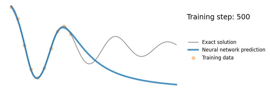
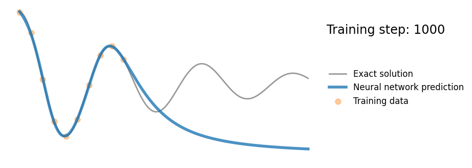
Normal (non-PINN) Neural Network

def plot_result(x,y,x_data,y_data,yh,xp=None):
    "Pretty plot training results"
    plt.figure(figsize=(8,4))
    plt.plot(x,y, color="grey", linewidth=2, alpha=0.8, label="Exact solution")
    plt.plot(x,yh, color="tab:blue", linewidth=4, alpha=0.8, label="Neural network prediction")
    plt.scatter(x_data, y_data, s=60, color="tab:orange", alpha=0.4, label='Training data')
    if xp is not None:
        plt.scatter(xp, -0*torch.ones_like(xp), s=60, color="tab:green", alpha=0.4, 
                    label='Physics loss training locations')
    l = plt.legend(loc=(1.01,0.34), frameon=False, fontsize="large")
    plt.setp(l.get_texts(), color="k")
    plt.xlim(-0.05, 1.05)
    plt.ylim(-1.1, 1.1)
    plt.text(1.065,0.7,"Training step: %i"%(i+1),fontsize="xx-large",color="k")
    plt.axis("off")
    
    
# train standard neural network to fit training data
torch.manual_seed(123)
model = FCN(1,1,32,3)
optimizer = torch.optim.Adam(model.parameters(),lr=1e-3)
files = []
for i in range(1000):
    optimizer.zero_grad()
    yh = model(x_data)
    loss = torch.mean((yh-y_data)**2)# use mean squared error
    loss.backward()
    optimizer.step()
    
    
    # plot the result as training progresses
    if (i+1) % 10 == 0: 
        
        yh = model(x).detach()
        
        plot_result(x,y,x_data,y_data,yh)
        
        file = "tmp_data/nn_%.8i.png"%(i+1)
        plt.savefig(file, bbox_inches='tight', pad_inches=0.1, dpi=100, facecolor="white")
        files.append(file)
    
        if (i+1) % 500 == 0: plt.show()
        else: plt.close("all")
            
save_gif_PIL("nn.gif", files, fps=20, loop=0)

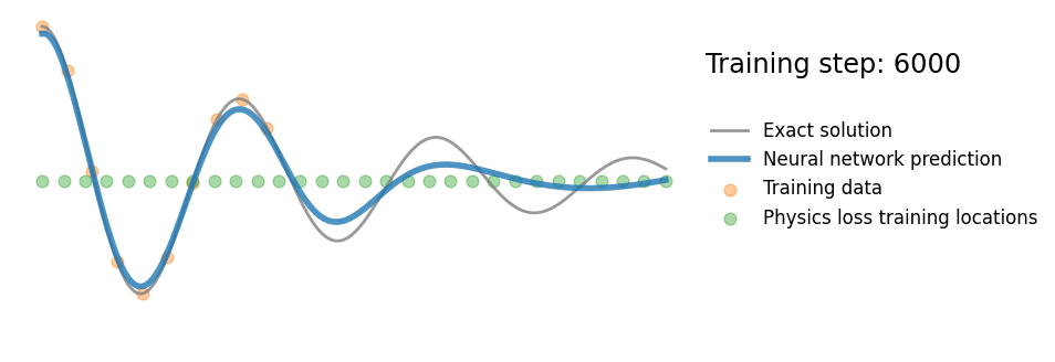
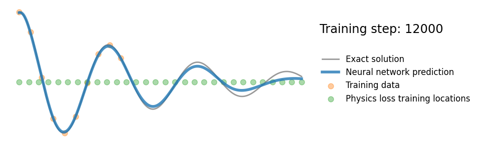
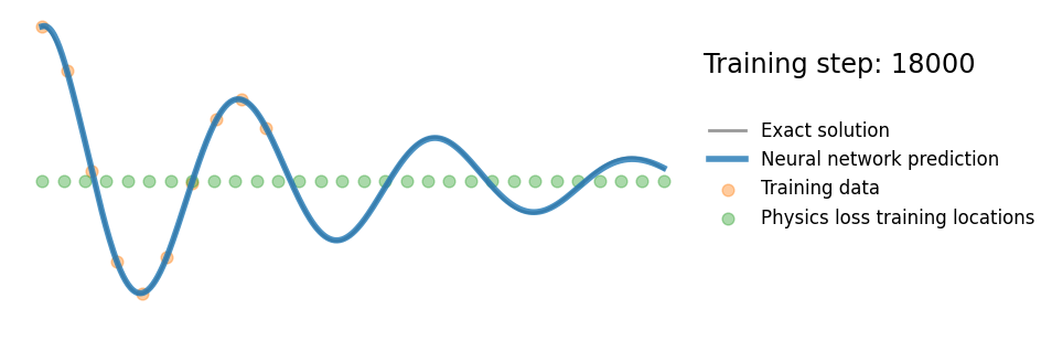
PINN

Finally, we add the underlying differential equation (“physics loss”) to the loss function.

The physics loss aims to ensure that the learned solution is consistent with the underlying differential equation. This is done by penalising the residual of the differential equation over a set of locations sampled from the domain.

Here we evaluate the physics loss at 30 points uniformly spaced over the problem domain \(([0,1])\). We can calculate the derivatives of the network solution with respect to its input variable at these points using pytorch’s autodifferentiation features, and can then easily compute the residual of the differential equation using these quantities.

x_physics = torch.linspace(0,1,30).view(-1,1).requires_grad_(True)# sample locations over the problem domain
mu, k = 2*d, w0**2

torch.manual_seed(123)
model = FCN(1,1,32,3)
optimizer = torch.optim.Adam(model.parameters(),lr=1e-4)
files = []
for i in range(20000):
    optimizer.zero_grad()
    
    # compute the "data loss"
    yh = model(x_data)
    loss1 = torch.mean((yh-y_data)**2)# use mean squared error
    
    # compute the "physics loss"
    yhp = model(x_physics)
    dx  = torch.autograd.grad(yhp, x_physics, torch.ones_like(yhp), create_graph=True)[0]# computes dy/dx
    dx2 = torch.autograd.grad(dx,  x_physics, torch.ones_like(dx),  create_graph=True)[0]# computes d^2y/dx^2
    physics = dx2 + mu*dx + k*yhp# computes the residual of the 1D harmonic oscillator differential equation
    loss2 = (1e-4)*torch.mean(physics**2)
    
    # backpropagate joint loss
    loss = loss1 + loss2# add two loss terms together
    loss.backward()
    optimizer.step()
    
    
    # plot the result as training progresses
    if (i+1) % 150 == 0: 
        
        yh = model(x).detach()
        xp = x_physics.detach()
        
        plot_result(x,y,x_data,y_data,yh,xp)
        
        file = "tmp_data/pinn_%.8i.png"%(i+1)
        plt.savefig(file, bbox_inches='tight', pad_inches=0.1, dpi=100, facecolor="white")
        files.append(file)
        
        if (i+1) % 6000 == 0: plt.show()
        else: plt.close("all")
            
save_gif_PIL("pinn.gif", files, fps=20, loop=0)

References

1. M. Raissi, P. Perdikaris, and G. E. Karniadakis. Physics-informed neural networks: A deep learning framework for solving forward and inverse problems involving nonlinear partial differential equations. Journal of Computational Physics, 378:686–707, February 2019.

2. George Em Karniadakis, Ioannis G. Kevrekidis, Lu Lu, Paris Perdikaris, Sifan Wang, and Liu Yang. Physics-informed machine learning. Nature Reviews Physics, 3(6):422–440, June 2021

Acknowledgments

• Initial version: Mark Neubauer

• 1D harmonic oscillator example is based on the blog post “So, what is a physics-informed neural network?”. This problem was inspired by the following blog post: https://beltoforion.de/en/harmonic_oscillator/.

© Copyright 2024