Vision Transformer#
import os
import subprocess
import torch
import torch.nn as nn
import numpy as np
import pandas as pd
from torch import optim
from torch.utils.data import Dataset, DataLoader
from torchvision.datasets import ImageFolder
from torchvision.transforms import Compose, Normalize, RandomHorizontalFlip, Resize, ToTensor
from transformers import get_cosine_schedule_with_warmup
from tqdm import tqdm
import matplotlib.pyplot as plt
import warnings; warnings.filterwarnings("ignore")
Overview#

Until a few years ago, Convolutions have been the default method of all Deep Learning for Vision tasks. But there was a limitation of the Convolution mechanism that prompted the creation of the Vision Transformer: Lack of Spatial Attention. More specifically, this means that Convolutions are able to model local features within the kernel size very well, but there was no way to explain how the top left part of an image is related to the bottom right.
The Transformer architecture was able to solve this for Sequence data, as the main goal is to learn the relationships between different pairs of words. In the same way, the goal of the Vision Transformer will be to learn how different parts of an image are related to one another.
Patch Embedding#
First we describe Patch Embedding, which is the main addition over the vanilla Transformer described in the Transformers notebook. The purpose of patch embeddings is to convert an Image into a “sequence” type data. To do so we will split an image into patches of size patch_size and encode each patch with a vector of length embed_dim.
Assume you have an image of size 3x224x224 and we want to use a patch_size of 16 and embed_dim of 768.
The number of patches can be calculated as \((\dfrac{224}{16})^2 = 196\). Therefore we want to get to the tensor of shape 196 x 768 where each patch is being represented with this embedding dimension.
We have two ways to do this:
Write a patching funciton to split our image of
3 x 224 x 224to a196 x 3 x 14 x 14. We can then flatten the last three dimensions and get a tensor of196 x 3 x 14 x 14and then use a linear layer to scale the3 x 14 x 14to our embed_dim.The prefered method will be to utilize the convolution mechanism in PyTorch to patch the image for us.
The convolution gives us the following inputs and we will fill them as such:
in_channels= 3 (We have RGB Images)out_channels= 768 (What is the embed dim we want?)kernel_size= 16 (How large do we want each patch?)stride = 16(If we dont want any overlapping patches our kernel size and stride have to be the same)
By doing this, we can essentially have a filter of size 16 traversing over our image with 16 pixel shifts, which will create 196 non-overlapping patches and return the tensor of shape
768 x 14 x 14. We will then flatten on the last dimension to get768 x 196and then transpose the tensor to get our final output of196 x 768.
class PatchEmbed(nn.Module):
    """
    PatchEmbed module will take an input image in the shape (C, H, W), patch the image into
    patches of size patch_size and embed each patch into embedding dim of embed_dim
    """
    def __init__(self, img_size=224, patch_size=16, in_chans=3, embed_dim=786):
        super(PatchEmbed, self).__init__()
        self.img_size = img_size
        self.patch_size = patch_size
        self.in_chans = in_chans
        self.embed_dim = embed_dim

        ### Calculate Number of Patches ###
        self.n_patches = (img_size // patch_size) ** 2

        ### Use Convolution to Patch the Images ###
        self.proj = nn.Conv2d(in_channels=in_chans,
                              out_channels=embed_dim,
                              kernel_size=patch_size,
                              stride=patch_size)

    def forward(self, x):
        x = self.proj(x) # (batch , embed_dim , sqrt(n_patches) , sqrt(n_patches))
        x = x.flatten(2) # (batch , embed_dim , n_patches)
        x = x.transpose(1,2) # (batch, n_patches, embed_dim)
        return x
Class Tokens and Positional Embeddings#
Unfortunately, Transformers have an issue of Permuation Invariance. What this means is, if we were doing an NLP task, the Transformer wouldn’t pay any attention to the order or words (which is obviously a problem for sequence tasks). Also, we need to be able to aggregate all the information across all the patches into a single vector that can then be used for classification at the end. We will codify these two things later when defining the final Vision Transformer but for now lets review the concept.
What we will do first is concatenate onto our original tensor of shape 196 x 768 and concatenate on some learnable parameters CLS_TOKEN of shape 1 x 768 to create our final data shape of 197 x 768. We will then add to this new tensor additional learnable parameters called the Positional Embeddings of the shape 197 x 768 that will learn to encode spatial (or temporal in sequence tasks) relationships.
Single Headed Attention#
To calculate attention we will have to generate three distinct projections of our data, known as the Queries, Keys and Values. The purpose of this is to use the Queries and Keys to create score weights between different patches of the image and then use that new weight matrix to perform something analogous to a weighted average of the Values matrix.
Step 1: Projection#
We will take our Input Data 197 x 768 that includes that CLS TOKEN and has the Positional Embeddings added to it and project it to three seperate tensors of the same shape. Essentially we are doing three seperate matrix multiplications on weight matricies \(W_Q\), \(W_K\) , \(W_V\) which is the same as doing a simple Linear layer. Because we want the shape to be the same, if we have an input embedding of 768, we will output the same 768, therefore using a Linear layer \(nn.Linear(768,768)\)
Step 2: Build the Attention Matrix#
We will multiply together our Queries and the Transpose of the Keys to generate a tensor of shape 197 x 197. More specifically, we have a matrix of (num_patches + 1) x (num_patches + 1) which will encode the relationship between each pair of patches.
Step 3: Normalize and Softmax#
Next we divide the resulting Attention matrix by the square root of our embedding length. It was shown that the variance of the attention matrix scaled higher with larger embedding lenghts so this is a simple normalization procedue to make sure the variance of our Q, K and Attention Matrix are all about the same.
More important is our softmax, to ensure that each row of our attention matrix adds to 1. This way, it turns the next calcualation into a simple weighted average of the values.
Step 4: Multiply with Values for Output#
We then take our Attention matrix of shape 197 x 197 and multiply it with our third projection, the Values with shape 197 x 768 giving us the final Output of shape 197 x 768. Notice that the output tensor shape of this entire Attention calculation is identical to the input shape! This allows us to quickly scale the model in the future.
Aside: Couple of Details on why its a Weighted Average#
Pretend our Attention matrix is of shape 3 x 3 and the values matrix is of shape 3 x 768. After performing softmax on our attention matrix, each row will sum to one. Therefore, when multiplying with the Values matrix, each row of the Attention martrix is encoding a weighted sum of the embeddings of the values matrix.
class Head(nn.Module):
    """
    Single Attention Head to calculate the Q, K, V and return the weighted average matrix via 3 linear layers
    """
    def __init__(self, embed_dim=768, head_dim=768, attn_p=0):
        super(Head, self).__init__()
        self.query = nn.Linear(embed_dim, head_dim)
        self.key = nn.Linear(embed_dim, head_dim)
        self.value = nn.Linear(embed_dim, head_dim)
        self.attn_dropout = nn.Dropout(attn_p)

    def forward(self, x):
        batch_size, n_patch, embed_dim = x.shape
        q = self.query(x) # (batch, n_patches+1, head_dim)
        k = self.key(x) # (batch, n_patches+1, head_dim)
        v = self.value(x) # (batch, n_patches+1, head_dim)

        sam = (q @ k.transpose(-2,-1)) * embed_dim**-0.5 # (batch , n_patches+1, n_patches+1)
        attn = sam.softmax(dim=-1) # (batch , n_patches+1, n_patches+1)
        attn = self.attn_dropout(attn)
        weighted_average = attn @ v # (batch , n_patches+1, head_dim)
        return weighted_average
Multi Headed Attention#
Multi Headed Attention only changes one aspect of all the previous ideas we explored. Instead of only have a single set of projections \(Q\), \(K\), \(V\) that take input tensor of shape 197 x 768 and project to a new tensor of the same shape 197 x 768, what if we do this multiple times?
The first step is to determine the number of heads we want, and lets say we want 12. This would indicate that the dimension of each head should be \((\dfrac{768}{12}) = 64\). Therefore, we want to take an input tensor of 197 x 768 and project it to a new tensor for the \(Q\), \(K\), and \(V\) of shape 197 x 64. Again we can do this with a simple linear layer, but instead of \(nn.Linear(768, 786)\) we will do \(nn.Linear(768, 64)\).
We wil then repeat this step 12 times with 12 unique triplets of linear layers and get 12 outputs each of shape 197 x 64. We can then concatenate all these back together to get the final shape 197 x 768, right back to where we started! The problem here though is we just concatenated the 12 attention heads together, but they never got a chance to share information across one another, therefore we will use another linear layer \(nn.Linear(768, 786)\) to perform some information meshing.
class MultiHeadedAttention(nn.Module):
    """
    Multiple Attention Head to repeat Head module num_heads times and concatenate outputs of heads together.
    """
    def __init__(self, embed_dim=768, num_heads=12, attn_p=0, proj_p=0):
        super(MultiHeadedAttention, self).__init__()
        self.head_size = embed_dim // num_heads
        self.heads = nn.ModuleList([Head(embed_dim=embed_dim, head_dim=self.head_size, attn_p=attn_p) for _ in range(num_heads)])
        self.proj = nn.Linear(embed_dim, embed_dim)
        self.proj_drop = nn.Dropout(proj_p)

    def forward(self, x):
        out = torch.cat([h(x) for h in self.heads], dim=-1) # (batch, n_patches+1, embed_dim)
        out = self.proj_drop(self.proj(out)) # (batch, n_patches+1, embed_dim)
        return out
Efficient Attention#
As we saw in our MultiHeaded Attention example, we are doing a for loop to pass our tensor through each head. We obviously would like to make this run in parallel so we can put the Attention Head and MultiHeaded Attention together. Another change is, instead of using three seperate linear layers for \(Q\), \(K\) and \(V\), we can actually just use a single linear layer \(nn.Linear(768, 3*786)\) that essentially outputs the same thing in a single weight matrix. We can then do some fun matrix manipulations to extract our \(Q\), \(K\) and \(V\) and do our attention calculations.
There is no good way to draw this, so step through the code below line by line and pay close attention to the shapes of each tensor.
class EfficientAttention(nn.Module):
    def __init__(self, embed_dim, num_heads, attn_p, proj_p):
        super(EfficientAttention, self).__init__()
        self.embed_dim = embed_dim
        self.num_heads = num_heads
        self.head_size = int(self.embed_dim / num_heads)

        self.qkv = nn.Linear(embed_dim, embed_dim*3)
        self.attn_dropout = nn.Dropout(attn_p)
        self.proj = nn.Linear(embed_dim, embed_dim)
        self.proj_drop = nn.Dropout(proj_p)

    def forward(self, x):
        batch, patches, embed_dim = x.shape # (batch, n_patches+1, embed_dim)
        qkv = self.qkv(x) # (batch, n_patches+1, 3*embed_dim)
        qkv = qkv.reshape(batch, patches, 3, self.num_heads, self.head_size) # (batch, patch+1, 3, num_heads, head_size)
        qkv = qkv.permute(2, 0, 3, 1, 4)  # (3, batch, num_heads, patches+1, head_size)
        q, k, v = qkv[0], qkv[1], qkv[2] # Each of shape (batch, num_heads, patches+1, head_size)

        ### SAME AS BEFORE NOW ###
        sam = (q @ k.transpose(-2,-1)) * self.head_size**-0.5 # (batch, num_heads, patches+1, patches+1)
        attn = sam.softmax(dim=-1)
        attn = self.attn_dropout(attn)
        weighted_average = attn @ v # (batch, num_heads, patches+1, head_size)
        weighted_average = weighted_average.transpose(1,2) # (batch, patches+1, num_heads, head_size)
        weighted_average = weighted_average.flatten(2) # (batch, patches+1, embed_dim)
        out = self.proj_drop(self.proj(weighted_average))
        return out
MultiLayer Percepteron#
As we can see from this small snippet of the image in the original Transformer paper, after performing our MultiHeaded attention calculation, we have a simple Feed Forward module. This is just a typical MLP with a few linear layers, and the only parameter is the mlp_ratio which we will specify a little later. The overview is if the input is of dimension 768, then we will have a hidden layer of size 768 * mlp_ratio and then another output layer that will bring it back to a dimension of 768.
class MLP(nn.Module):
    def __init__(self, in_features, hidden_features, out_features, mlp_p=0):
        """
        Hidden features should be some MLP_ratio * in_features.
        Out Features == In Features
        """
        super(MLP, self).__init__()
        self.fc1 = nn.Linear(in_features, hidden_features)
        self.act = nn.GELU()
        self.fc2 = nn.Linear(hidden_features, out_features)
        self.drop = nn.Dropout(mlp_p)

    def forward(self, x):
        x = self.act(self.fc1(x)) # (batch, n_patches+1, embed_dim * mlp_ratio)
        x = self.drop(x)
        x = self.fc2(x) # (batch, n_patches+1, embed_dim)
        x = self.drop(x)
        return x
Putting Together the Transformer Block#
In this step we will add in all parts we have build previously together in a transformer block, using Residual Connections and Layer Normalization for the reasons discussed in the Transformers notebook.
class TransformerBlock(nn.Module):
    """
    Full Transformer block with Attention and Linear Layers
    """
    def __init__(self, embed_dim=768, num_heads=12, mlp_ratio=4.0,
                 mlp_p=0, attn_p=0, proj_p=0, efficient=True):
        super(TransformerBlock, self).__init__()
        self.norm1 = nn.LayerNorm(embed_dim, eps=1e-6)

        if efficient:
            self.attn = EfficientAttention(embed_dim=embed_dim,
                                           num_heads=num_heads,
                                           attn_p=attn_p,
                                           proj_p=proj_p)
        else:
            self.attn = MultiHeadedAttention(embed_dim=embed_dim,
                                             num_heads=num_heads,
                                             attn_p=attn_p,
                                             proj_p=proj_p)

        self.norm2 = nn.LayerNorm(embed_dim, eps=1e-6)
        hidden_features = int(embed_dim*mlp_ratio)
        self.mlp = MLP(in_features=embed_dim,
                       hidden_features=hidden_features,
                       out_features=embed_dim,
                       mlp_p=mlp_p)

    def forward(self, x):
        """
        Residual connections to avoid vanishing gradients (notice its is X = X + Out rather than doing X = Out)
        """
        x = x + self.attn(self.norm1(x)) # (batch, n_patches+1, embed_dim)
        x = x + self.mlp(self.norm2(x)) # (batch, n_patches+1, embed_dim)
        return x
Putting Together the Vision Transformer#
In this next step we will put together all the parts for the Vision Transformer. There are a few new things included that we talked about previously.
This is where we will instantiate the CLS_TOKEN of shape 1 x 768 to concatenate onto our samples and the Positional Embeddings of shape 197 x 768. We want the same values of the CLS tokens to be concatenated onto each sample in a batch so each image can have its own unique calculations on it so we will have to expand the dimension to match the batch size in the forward fuction. The Positional Embeddings on the other hand can just be directly added as we want the same positional encoding regardless of the image.
Input Shape = Output Shape#
I have been making a big deal about the shapes of tensors, and the reason is the unique part of the Transformer Architecture, is the input shape of the transformer block is identical to the output shape. This means we can just stack a bunch of MultiHeaded attention blocks on top of each other and not worry about shape errors. (Rember in convolutions, the shapes can be really hard to match sometimes so this is a huge annoyance saver!)
Classification Task#
Once we are at the end, we will strip out only the CLS tokens and use that for prediction to our N_classes. In our case we will do Dogs vs Cats so that will be two Classes. In the image here I show that I strip of the bottom because I concatenated the cls tokens to the bottom, but in the implemenation it is concatenated to the top! Regardless the idea is the same
class VisionTransformer(nn.Module):
    """
    VisionTransfomrer put together. Main parameters to change are:
    img_size: Size of input image
    patch_size:  Size of individual patches (Smaller patches lead to more patches)
    n_classes: Number of outputs for classification
    embed_dim: Length of embedding vector for each patch
    depth: Number of wanted transformer blocks
    num_heads: Number of wanted attention heads per block
    """
    def __init__(self, img_size=224, patch_size=16, in_chans=3, n_classes=2,
                 embed_dim=768, depth=12, num_heads=12, mlp_ratio=4, attn_p=0.2,
                 mlp_p=0.2, proj_p=0.2, pos_drop=0.2, efficient=True):
        super(VisionTransformer, self).__init__()

        self.patch_embed = PatchEmbed(img_size=img_size,
                                      patch_size=patch_size,
                                      in_chans=in_chans,
                                      embed_dim=embed_dim)

        self.cls_token = nn.Parameter(torch.zeros(1,1,embed_dim))
        self.pos_embed = nn.Parameter((torch.zeros(1, 1+self.patch_embed.n_patches, embed_dim)))
        self.pos_drop = nn.Dropout(pos_drop)

        self.blocks = nn.ModuleList(
            [
                TransformerBlock(embed_dim=embed_dim,
                                 num_heads=num_heads,
                                 mlp_ratio=mlp_ratio,
                                 mlp_p=mlp_p,
                                 attn_p=attn_p,
                                 proj_p=proj_p,
                                 efficient=efficient)
                for _ in range(depth)
            ]
        )

        self.norm = nn.LayerNorm(embed_dim, eps=1e-6)
        self.head = nn.Linear(embed_dim, n_classes)

    def forward(self, x):
        batch_size = x.shape[0]
        x = self.patch_embed(x) # (batch, n_patches, embed_dim)
        cls_token = self.cls_token.expand(batch_size, -1, -1) # (batch, 1, embed_dim)
        x = torch.cat((cls_token, x), dim=1) # (batch, n_patches+1, embed_dim)
        x = x + self.pos_embed
        x = self.pos_drop(x)

        for block in self.blocks:
            x = block(x)

        x = self.norm(x)
        cls_token_final = x[:, 0] # (batch, embed_dim)
        x = self.head(cls_token_final) # (batch, n_classes)
        return x, cls_token_final
Training Script#
At this point everything is done and we just need to train the model!
def train(model, device, epochs, optimizer,
          scheduler, loss_fn, trainloader,
          valloader, savepath="./tmp_data/ViTDogsvCatsSmall.pt"):
    log_training = {"epoch": [],
                    "training_loss": [],
                    "training_acc": [],
                    "validation_loss": [],
                    "validation_acc": []}

    best_val_loss = np.inf
    for epoch in range(1, epochs + 1):
        print(f"Starting Epoch {epoch}")
        training_losses, training_accuracies = [], []
        validation_losses, validation_accuracies = [], []

        for image, label in tqdm(trainloader):
            image, label = image.to(device), label.to(device)
            optimizer.zero_grad()
            out, _ = model.forward(image)

            ### CALCULATE LOSS ##
            loss = loss_fn(out, label)
            training_losses.append(loss.item())

            ### CALCULATE ACCURACY ###
            predictions = torch.argmax(out, axis=1)
            accuracy = (predictions == label).sum() / len(predictions)
            training_accuracies.append(accuracy.item())

            loss.backward()
            optimizer.step()
            scheduler.step()

        for image, label in tqdm(valloader):
            image, label = image.to(device), label.to(device)
            with torch.no_grad():
                out, _ = model.forward(image)

                ### CALCULATE LOSS ##
                loss = loss_fn(out, label)
                validation_losses.append(loss.item())

                ### CALCULATE ACCURACY ###
                predictions = torch.argmax(out, axis=1)
                accuracy = (predictions == label).sum() / len(predictions)
                validation_accuracies.append(accuracy.item())

        training_loss_mean, training_acc_mean = np.mean(training_losses), np.mean(training_accuracies)
        valid_loss_mean, valid_acc_mean = np.mean(validation_losses), np.mean(validation_accuracies)

        ### Save Model If Val Loss Decreases ###
        if valid_loss_mean < best_val_loss:
            print("---Saving Model---")
            torch.save(model.state_dict(), savepath)
            best_val_loss = valid_loss_mean

        log_training["epoch"].append(epoch)
        log_training["training_loss"].append(training_loss_mean)
        log_training["training_acc"].append(training_acc_mean)
        log_training["validation_loss"].append(valid_loss_mean)
        log_training["validation_acc"].append(valid_acc_mean)


        print("Training Loss:", training_loss_mean)
        print("Training Acc:", training_acc_mean)
        print("Validation Loss:", valid_loss_mean)
        print("Validation Acc:", valid_acc_mean)

    return log_training, model
def wget_data(url: str, local_path='./tmp_data'):
  os.makedirs(local_path, exist_ok=True)

  p = subprocess.Popen(["wget", "-nc", "-P", local_path, url], stderr=subprocess.PIPE, encoding='UTF-8')
  rc = None

  while rc is None:
    line = p.stderr.readline().strip('\n')
    if len(line) > 0:
      print(line)
    rc = p.poll()
Get Pet dataset#
wget_data('https://courses.physics.illinois.edu/phys503/fa2023/data/kagglecatsanddogs_5340.zip')
--2026-03-09 12:53:24-- https://courses.physics.illinois.edu/phys503/fa2023/data/kagglecatsanddogs_5340.zip
Resolving courses.physics.illinois.edu (courses.physics.illinois.edu)... 130.126.151.14
Connecting to courses.physics.illinois.edu (courses.physics.illinois.edu)|130.126.151.14|:443... connected.
HTTP request sent, awaiting response... 200 OK
Length: 824887076 (787M) [application/x-zip-compressed]
Saving to: ‘./tmp_data/kagglecatsanddogs_5340.zip’
0K .......... .......... .......... .......... .......... 0% 1.34M 9m47s
50K .......... .......... .......... .......... .......... 0% 1.56M 9m6s
100K .......... .......... .......... .......... .......... 0% 3.69M 7m15s
150K .......... .......... .......... .......... .......... 0% 1.60M 7m29s
200K .......... .......... .......... .......... .......... 0% 18.9M 6m7s
250K .......... .......... .......... .......... .......... 0% 24.6M 5m12s
300K .......... .......... .......... .......... .......... 0% 2.43M 5m13s
350K .......... .......... .......... .......... .......... 0% 3.36M 5m3s
400K .......... .......... .......... .......... .......... 0% 7.53M 4m41s
450K .......... .......... .......... .......... .......... 0% 65.9M 4m14s
500K .......... .......... .......... .......... .......... 0% 9.07M 3m59s
550K .......... .......... .......... .......... .......... 0% 46.7M 3m40s
600K .......... .......... .......... .......... .......... 0% 11.0M 3m29s
650K .......... .......... .......... .......... .......... 0% 121M 3m15s
700K .......... .......... .......... .......... .......... 0% 3.96M 3m15s
750K .......... .......... .......... .......... .......... 0% 36.5M 3m4s
800K .......... .......... .......... .......... .......... 0% 2.91M 3m9s
850K .......... .......... .......... .......... .......... 0% 3.63M 3m11s
900K .......... .......... .......... .......... .......... 0% 37.3M 3m2s
950K .......... .......... .......... .......... .......... 0% 8.33M 2m57s
1000K .......... .......... .......... .......... .......... 0% 13.9M 2m51s
1050K .......... .......... .......... .......... .......... 0% 22.7M 2m45s
1100K .......... .......... .......... .......... .......... 0% 47.7M 2m39s
1150K .......... .......... .......... .......... .......... 0% 4.64M 2m39s
1200K .......... .......... .......... .......... .......... 0% 34.4M 2m34s
1250K .......... .......... .......... .......... .......... 0% 22.3M 2m29s
1300K .......... .......... .......... .......... .......... 0% 28.4M 2m25s
1350K .......... .......... .......... .......... .......... 0% 22.4M 2m21s
1400K .......... .......... .......... .......... .......... 0% 18.2M 2m17s
1450K .......... .......... .......... .......... .......... 0% 124M 2m13s
1500K .......... .......... .......... .......... .......... 0% 19.0M 2m10s
1550K .......... .......... .......... .......... .......... 0% 45.6M 2m6s
1600K .......... .......... .......... .......... .......... 0% 14.2M 2m4s
1650K .......... .......... .......... .......... .......... 0% 15.6M 2m2s
1700K .......... .......... .......... .......... .......... 0% 40.4M 1m59s
1750K .......... .......... .......... .......... .......... 0% 90.9M 1m56s
1800K .......... .......... .......... .......... .......... 0% 29.6M 1m54s
1850K .......... .......... .......... .......... .......... 0% 26.4M 1m51s
1900K .......... .......... .......... .......... .......... 0% 26.9M 1m49s
1950K .......... .......... .......... .......... .......... 0% 14.5M 1m48s
2000K .......... .......... .......... .......... .......... 0% 7.08M 1m48s
2050K .......... .......... .......... .......... .......... 0% 15.9M 1m47s
2100K .......... .......... .......... .......... .......... 0% 9.45M 1m46s
2150K .......... .......... .......... .......... .......... 0% 8.47M 1m46s
2200K .......... .......... .......... .......... .......... 0% 12.4M 1m45s
2250K .......... .......... .......... .......... .......... 0% 14.0M 1m44s
2300K .......... .......... .......... .......... .......... 0% 20.8M 1m42s
2350K .......... .......... .......... .......... .......... 0% 26.9M 1m41s
2400K .......... .......... .......... .......... .......... 0% 11.9M 1m40s
2450K .......... .......... .......... .......... .......... 0% 23.5M 99s
2500K .......... .......... .......... .......... .......... 0% 13.3M 98s
2550K .......... .......... .......... .......... .......... 0% 23.4M 97s
2600K .......... .......... .......... .......... .......... 0% 21.7M 96s
2650K .......... .......... .......... .......... .......... 0% 18.6M 95s
2700K .......... .......... .......... .......... .......... 0% 25.2M 93s
2750K .......... .......... .......... .......... .......... 0% 22.2M 92s
2800K .......... .......... .......... .......... .......... 0% 7.56M 93s
2850K .......... .......... .......... .......... .......... 0% 19.1M 92s
2900K .......... .......... .......... .......... .......... 0% 20.7M 91s
2950K .......... .......... .......... .......... .......... 0% 23.3M 90s
3000K .......... .......... .......... .......... .......... 0% 10.7M 90s
3050K .......... .......... .......... .......... .......... 0% 8.52M 90s
3100K .......... .......... .......... .......... .......... 0% 50.7M 88s
3150K .......... .......... .......... .......... .......... 0% 20.8M 88s
3200K .......... .......... .......... .......... .......... 0% 15.5M 87s
3250K .......... .......... .......... .......... .......... 0% 22.5M 86s
3300K .......... .......... .......... .......... .......... 0% 16.2M 86s
3350K .......... .......... .......... .......... .......... 0% 38.8M 85s
3400K .......... .......... .......... .......... .......... 0% 13.1M 84s
3450K .......... .......... .......... .......... .......... 0% 19.3M 84s
3500K .......... .......... .......... .......... .......... 0% 23.4M 83s
3550K .......... .......... .......... .......... .......... 0% 50.2M 82s
3600K .......... .......... .......... .......... .......... 0% 14.1M 82s
3650K .......... .......... .......... .......... .......... 0% 38.4M 81s
3700K .......... .......... .......... .......... .......... 0% 16.8M 80s
3750K .......... .......... .......... .......... .......... 0% 39.7M 80s
3800K .......... .......... .......... .......... .......... 0% 21.5M 79s
3850K .......... .......... .......... .......... .......... 0% 28.4M 78s
3900K .......... .......... .......... .......... .......... 0% 16.8M 78s
3950K .......... .......... .......... .......... .......... 0% 44.1M 77s
4000K .......... .......... .......... .......... .......... 0% 18.4M 77s
4050K .......... .......... .......... .......... .......... 0% 12.1M 77s
4100K .......... .......... .......... .......... .......... 0% 90.8M 76s
4150K .......... .......... .......... .......... .......... 0% 16.1M 75s
4200K .......... .......... .......... .......... .......... 0% 4.36M 77s
4250K .......... .......... .......... .......... .......... 0% 3.68M 78s
4300K .......... .......... .......... .......... .......... 0% 7.46M 79s
4350K .......... .......... .......... .......... .......... 0% 8.21M 79s
4400K .......... .......... .......... .......... .......... 0% 3.28M 80s
4450K .......... .......... .......... .......... .......... 0% 21.2M 80s
4500K .......... .......... .......... .......... .......... 0% 17.8M 80s
4550K .......... .......... .......... .......... .......... 0% 5.29M 80s
4600K .......... .......... .......... .......... .......... 0% 20.5M 80s
4650K .......... .......... .......... .......... .......... 0% 13.5M 80s
4700K .......... .......... .......... .......... .......... 0% 22.6M 79s
4750K .......... .......... .......... .......... .......... 0% 29.3M 79s
4800K .......... .......... .......... .......... .......... 0% 18.2M 78s
4850K .......... .......... .......... .......... .......... 0% 19.7M 78s
4900K .......... .......... .......... .......... .......... 0% 25.6M 77s
4950K .......... .......... .......... .......... .......... 0% 24.2M 77s
5000K .......... .......... .......... .......... .......... 0% 24.9M 76s
5050K .......... .......... .......... .......... .......... 0% 19.6M 76s
5100K .......... .......... .......... .......... .......... 0% 12.8M 76s
5150K .......... .......... .......... .......... .......... 0% 186M 75s
5200K .......... .......... .......... .......... .......... 0% 9.06M 75s
5250K .......... .......... .......... .......... .......... 0% 13.4M 75s
5300K .......... .......... .......... .......... .......... 0% 22.0M 75s
5350K .......... .......... .......... .......... .......... 0% 12.8M 75s
5400K .......... .......... .......... .......... .......... 0% 20.2M 74s
5450K .......... .......... .......... .......... .......... 0% 8.40M 74s
5500K .......... .......... .......... .......... .......... 0% 34.1M 74s
5550K .......... .......... .......... .......... .......... 0% 6.02M 75s
5600K .......... .......... .......... .......... .......... 0% 7.52M 75s
5650K .......... .......... .......... .......... .......... 0% 13.3M 75s
5700K .......... .......... .......... .......... .......... 0% 19.2M 74s
5750K .......... .......... .......... .......... .......... 0% 14.9M 74s
5800K .......... .......... .......... .......... .......... 0% 7.18M 74s
5850K .......... .......... .......... .......... .......... 0% 31.8M 74s
5900K .......... .......... .......... .......... .......... 0% 15.1M 74s
5950K .......... .......... .......... .......... .......... 0% 75.8M 73s
6000K .......... .......... .......... .......... .......... 0% 16.3M 73s
6050K .......... .......... .......... .......... .......... 0% 24.1M 73s
6100K .......... .......... .......... .......... .......... 0% 15.4M 73s
6150K .......... .......... .......... .......... .......... 0% 27.2M 72s
6200K .......... .......... .......... .......... .......... 0% 16.3M 72s
6250K .......... .......... .......... .......... .......... 0% 25.0M 72s
6300K .......... .......... .......... .......... .......... 0% 33.5M 71s
6350K .......... .......... .......... .......... .......... 0% 14.8M 71s
6400K .......... .......... .......... .......... .......... 0% 6.88M 71s
6450K .......... .......... .......... .......... .......... 0% 11.4M 71s
6500K .......... .......... .......... .......... .......... 0% 21.2M 71s
6550K .......... .......... .......... .......... .......... 0% 11.6M 71s
6600K .......... .......... .......... .......... .......... 0% 18.3M 71s
6650K .......... .......... .......... .......... .......... 0% 9.68M 71s
6700K .......... .......... .......... .......... .......... 0% 15.2M 71s
6750K .......... .......... .......... .......... .......... 0% 69.5M 70s
6800K .......... .......... .......... .......... .......... 0% 16.5M 70s
6850K .......... .......... .......... .......... .......... 0% 11.4M 70s
6900K .......... .......... .......... .......... .......... 0% 50.5M 70s
6950K .......... .......... .......... .......... .......... 0% 23.7M 70s
7000K .......... .......... .......... .......... .......... 0% 22.6M 69s
7050K .......... .......... .......... .......... .......... 0% 13.3M 69s
7100K .......... .......... .......... .......... .......... 0% 27.4M 69s
7150K .......... .......... .......... .......... .......... 0% 23.8M 69s
7200K .......... .......... .......... .......... .......... 0% 10.4M 69s
7250K .......... .......... .......... .......... .......... 0% 22.6M 68s
7300K .......... .......... .......... .......... .......... 0% 15.9M 68s
7350K .......... .......... .......... .......... .......... 0% 35.4M 68s
7400K .......... .......... .......... .......... .......... 0% 18.4M 68s
7450K .......... .......... .......... .......... .......... 0% 22.4M 68s
7500K .......... .......... .......... .......... .......... 0% 21.6M 67s
7550K .......... .......... .......... .......... .......... 0% 11.6M 67s
7600K .......... .......... .......... .......... .......... 0% 8.27M 68s
7650K .......... .......... .......... .......... .......... 0% 22.7M 67s
7700K .......... .......... .......... .......... .......... 0% 22.7M 67s
7750K .......... .......... .......... .......... .......... 0% 13.4M 67s
7800K .......... .......... .......... .......... .......... 0% 37.2M 67s
7850K .......... .......... .......... .......... .......... 0% 22.8M 67s
7900K .......... .......... .......... .......... .......... 0% 22.3M 66s
7950K .......... .......... .......... .......... .......... 0% 17.4M 66s
8000K .......... .......... .......... .......... .......... 0% 16.3M 66s
8050K .......... .......... .......... .......... .......... 1% 22.3M 66s
8100K .......... .......... .......... .......... .......... 1% 11.6M 66s
8150K .......... .......... .......... .......... .......... 1% 12.9M 66s
8200K .......... .......... .......... .......... .......... 1% 91.8M 65s
8250K .......... .......... .......... .......... .......... 1% 22.6M 65s
8300K .......... .......... .......... .......... .......... 1% 20.1M 65s
8350K .......... .......... .......... .......... .......... 1% 21.8M 65s
8400K .......... .......... .......... .......... .......... 1% 16.3M 65s
8450K .......... .......... .......... .......... .......... 1% 16.6M 65s
8500K .......... .......... .......... .......... .......... 1% 22.3M 65s
8550K .......... .......... .......... .......... .......... 1% 20.3M 64s
8600K .......... .......... .......... .......... .......... 1% 26.4M 64s
8650K .......... .......... .......... .......... .......... 1% 12.7M 64s
8700K .......... .......... .......... .......... .......... 1% 48.9M 64s
8750K .......... .......... .......... .......... .......... 1% 22.0M 64s
8800K .......... .......... .......... .......... .......... 1% 11.1M 64s
8850K .......... .......... .......... .......... .......... 1% 22.3M 64s
8900K .......... .......... .......... .......... .......... 1% 22.4M 63s
8950K .......... .......... .......... .......... .......... 1% 22.3M 63s
9000K .......... .......... .......... .......... .......... 1% 18.3M 63s
9050K .......... .......... .......... .......... .......... 1% 22.0M 63s
9100K .......... .......... .......... .......... .......... 1% 21.3M 63s
9150K .......... .......... .......... .......... .......... 1% 23.8M 63s
9200K .......... .......... .......... .......... .......... 1% 9.45M 63s
9250K .......... .......... .......... .......... .......... 1% 15.5M 63s
9300K .......... .......... .......... .......... .......... 1% 20.2M 63s
9350K .......... .......... .......... .......... .......... 1% 44.9M 62s
9400K .......... .......... .......... .......... .......... 1% 32.1M 62s
9450K .......... .......... .......... .......... .......... 1% 27.3M 62s
9500K .......... .......... .......... .......... .......... 1% 17.9M 62s
9550K .......... .......... .......... .......... .......... 1% 7.50M 62s
9600K .......... .......... .......... .......... .......... 1% 15.9M 62s
9650K .......... .......... .......... .......... .......... 1% 35.3M 62s
9700K .......... .......... .......... .......... .......... 1% 15.6M 62s
9750K .......... .......... .......... .......... .......... 1% 23.7M 62s
9800K .......... .......... .......... .......... .......... 1% 37.4M 61s
9850K .......... .......... .......... .......... .......... 1% 17.3M 61s
9900K .......... .......... .......... .......... .......... 1% 47.8M 61s
9950K .......... .......... .......... .......... .......... 1% 23.0M 61s
10000K .......... .......... .......... .......... .......... 1% 17.9M 61s
10050K .......... .......... .......... .......... .......... 1% 24.7M 61s
10100K .......... .......... .......... .......... .......... 1% 21.2M 61s
10150K .......... .......... .......... .......... .......... 1% 9.36M 61s
10200K .......... .......... .......... .......... .......... 1% 62.0M 60s
10250K .......... .......... .......... .......... .......... 1% 24.4M 60s
10300K .......... .......... .......... .......... .......... 1% 21.3M 60s
10350K .......... .......... .......... .......... .......... 1% 21.2M 60s
10400K .......... .......... .......... .......... .......... 1% 13.4M 60s
10450K .......... .......... .......... .......... .......... 1% 58.1M 60s
10500K .......... .......... .......... .......... .......... 1% 24.7M 60s
10550K .......... .......... .......... .......... .......... 1% 22.5M 60s
10600K .......... .......... .......... .......... .......... 1% 23.9M 59s
10650K .......... .......... .......... .......... .......... 1% 25.2M 59s
10700K .......... .......... .......... .......... .......... 1% 25.0M 59s
10750K .......... .......... .......... .......... .......... 1% 15.0M 59s
10800K .......... .......... .......... .......... .......... 1% 16.4M 59s
10850K .......... .......... .......... .......... .......... 1% 11.4M 59s
10900K .......... .......... .......... .......... .......... 1% 17.9M 59s
10950K .......... .......... .......... .......... .......... 1% 44.7M 59s
11000K .......... .......... .......... .......... .......... 1% 24.0M 59s
11050K .......... .......... .......... .......... .......... 1% 18.1M 59s
11100K .......... .......... .......... .......... .......... 1% 22.4M 58s
11150K .......... .......... .......... .......... .......... 1% 23.4M 58s
11200K .......... .......... .......... .......... .......... 1% 17.3M 58s
11250K .......... .......... .......... .......... .......... 1% 21.0M 58s
11300K .......... .......... .......... .......... .......... 1% 18.7M 58s
11350K .......... .......... .......... .......... .......... 1% 22.1M 58s
11400K .......... .......... .......... .......... .......... 1% 9.30M 58s
11450K .......... .......... .......... .......... .......... 1% 28.0M 58s
11500K .......... .......... .......... .......... .......... 1% 18.7M 58s
11550K .......... .......... .......... .......... .......... 1% 19.2M 58s
11600K .......... .......... .......... .......... .......... 1% 5.38M 58s
11650K .......... .......... .......... .......... .......... 1% 50.1M 58s
11700K .......... .......... .......... .......... .......... 1% 18.0M 58s
11750K .......... .......... .......... .......... .......... 1% 33.4M 58s
11800K .......... .......... .......... .......... .......... 1% 25.1M 58s
11850K .......... .......... .......... .......... .......... 1% 16.7M 58s
11900K .......... .......... .......... .......... .......... 1% 47.8M 57s
11950K .......... .......... .......... .......... .......... 1% 11.9M 57s
12000K .......... .......... .......... .......... .......... 1% 40.8M 57s
12050K .......... .......... .......... .......... .......... 1% 25.8M 57s
12100K .......... .......... .......... .......... .......... 1% 25.7M 57s
12150K .......... .......... .......... .......... .......... 1% 17.8M 57s
12200K .......... .......... .......... .......... .......... 1% 25.8M 57s
12250K .......... .......... .......... .......... .......... 1% 22.7M 57s
12300K .......... .......... .......... .......... .......... 1% 28.4M 57s
12350K .......... .......... .......... .......... .......... 1% 12.7M 57s
12400K .......... .......... .......... .......... .......... 1% 11.4M 57s
12450K .......... .......... .......... .......... .......... 1% 40.8M 57s
12500K .......... .......... .......... .......... .......... 1% 19.0M 57s
12550K .......... .......... .......... .......... .......... 1% 24.9M 56s
12600K .......... .......... .......... .......... .......... 1% 24.0M 56s
12650K .......... .......... .......... .......... .......... 1% 17.1M 56s
12700K .......... .......... .......... .......... .......... 1% 18.5M 56s
12750K .......... .......... .......... .......... .......... 1% 69.9M 56s
12800K .......... .......... .......... .......... .......... 1% 18.6M 56s
12850K .......... .......... .......... .......... .......... 1% 22.2M 56s
12900K .......... .......... .......... .......... .......... 1% 30.9M 56s
12950K .......... .......... .......... .......... .......... 1% 8.05M 56s
13000K .......... .......... .......... .......... .......... 1% 7.65M 56s
13050K .......... .......... .......... .......... .......... 1% 16.6M 56s
13100K .......... .......... .......... .......... .......... 1% 30.6M 56s
13150K .......... .......... .......... .......... .......... 1% 12.9M 56s
13200K .......... .......... .......... .......... .......... 1% 19.3M 56s
13250K .......... .......... .......... .......... .......... 1% 12.5M 56s
13300K .......... .......... .......... .......... .......... 1% 20.5M 56s
13350K .......... .......... .......... .......... .......... 1% 18.5M 56s
13400K .......... .......... .......... .......... .......... 1% 16.4M 56s
13450K .......... .......... .......... .......... .......... 1% 7.34M 56s
13500K .......... .......... .......... .......... .......... 1% 17.0M 56s
13550K .......... .......... .......... .......... .......... 1% 33.1M 56s
13600K .......... .......... .......... .......... .......... 1% 16.8M 56s
13650K .......... .......... .......... .......... .......... 1% 15.3M 56s
13700K .......... .......... .......... .......... .......... 1% 22.3M 56s
13750K .......... .......... .......... .......... .......... 1% 21.7M 56s
13800K .......... .......... .......... .......... .......... 1% 9.79M 56s
13850K .......... .......... .......... .......... .......... 1% 25.1M 56s
13900K .......... .......... .......... .......... .......... 1% 21.6M 55s
13950K .......... .......... .......... .......... .......... 1% 22.0M 55s
14000K .......... .......... .......... .......... .......... 1% 13.5M 55s
14050K .......... .......... .......... .......... .......... 1% 22.8M 55s
14100K .......... .......... .......... .......... .......... 1% 20.4M 55s
14150K .......... .......... .......... .......... .......... 1% 16.0M 55s
14200K .......... .......... .......... .......... .......... 1% 24.5M 55s
14250K .......... .......... .......... .......... .......... 1% 21.7M 55s
14300K .......... .......... .......... .......... .......... 1% 22.7M 55s
14350K .......... .......... .......... .......... .......... 1% 17.4M 55s
14400K .......... .......... .......... .......... .......... 1% 17.6M 55s
14450K .......... .......... .......... .......... .......... 1% 23.4M 55s
14500K .......... .......... .......... .......... .......... 1% 15.9M 55s
14550K .......... .......... .......... .......... .......... 1% 21.4M 55s
14600K .......... .......... .......... .......... .......... 1% 21.7M 55s
14650K .......... .......... .......... .......... .......... 1% 22.6M 55s
14700K .......... .......... .......... .......... .......... 1% 15.1M 55s
14750K .......... .......... .......... .......... .......... 1% 30.3M 54s
14800K .......... .......... .......... .......... .......... 1% 16.3M 54s
14850K .......... .......... .......... .......... .......... 1% 9.27M 55s
14900K .......... .......... .......... .......... .......... 1% 65.8M 54s
14950K .......... .......... .......... .......... .......... 1% 24.1M 54s
15000K .......... .......... .......... .......... .......... 1% 22.4M 54s
15050K .......... .......... .......... .......... .......... 1% 18.5M 54s
15100K .......... .......... .......... .......... .......... 1% 15.7M 54s
15150K .......... .......... .......... .......... .......... 1% 43.5M 54s
15200K .......... .......... .......... .......... .......... 1% 16.2M 54s
15250K .......... .......... .......... .......... .......... 1% 20.0M 54s
15300K .......... .......... .......... .......... .......... 1% 26.6M 54s
15350K .......... .......... .......... .......... .......... 1% 24.5M 54s
15400K .......... .......... .......... .......... .......... 1% 7.08M 54s
15450K .......... .......... .......... .......... .......... 1% 23.0M 54s
15500K .......... .......... .......... .......... .......... 1% 15.7M 54s
15550K .......... .......... .......... .......... .......... 1% 53.2M 54s
15600K .......... .......... .......... .......... .......... 1% 15.2M 54s
15650K .......... .......... .......... .......... .......... 1% 35.3M 54s
15700K .......... .......... .......... .......... .......... 1% 24.8M 54s
15750K .......... .......... .......... .......... .......... 1% 25.7M 53s
15800K .......... .......... .......... .......... .......... 1% 17.3M 53s
15850K .......... .......... .......... .......... .......... 1% 35.0M 53s
15900K .......... .......... .......... .......... .......... 1% 18.4M 53s
15950K .......... .......... .......... .......... .......... 1% 26.5M 53s
16000K .......... .......... .......... .......... .......... 1% 13.4M 53s
16050K .......... .......... .......... .......... .......... 1% 24.0M 53s
16100K .......... .......... .......... .......... .......... 2% 25.7M 53s
16150K .......... .......... .......... .......... .......... 2% 24.2M 53s
16200K .......... .......... .......... .......... .......... 2% 10.9M 53s
16250K .......... .......... .......... .......... .......... 2% 42.4M 53s
16300K .......... .......... .......... .......... .......... 2% 15.4M 53s
16350K .......... .......... .......... .......... .......... 2% 17.6M 53s
16400K .......... .......... .......... .......... .......... 2% 14.3M 53s
16450K .......... .......... .......... .......... .......... 2% 41.9M 53s
16500K .......... .......... .......... .......... .......... 2% 13.7M 53s
16550K .......... .......... .......... .......... .......... 2% 12.5M 53s
16600K .......... .......... .......... .......... .......... 2% 25.8M 53s
16650K .......... .......... .......... .......... .......... 2% 12.5M 53s
16700K .......... .......... .......... .......... .......... 2% 71.5M 53s
16750K .......... .......... .......... .......... .......... 2% 26.4M 53s
16800K .......... .......... .......... .......... .......... 2% 18.7M 53s
16850K .......... .......... .......... .......... .......... 2% 13.8M 53s
16900K .......... .......... .......... .......... .......... 2% 49.9M 52s
16950K .......... .......... .......... .......... .......... 2% 12.7M 52s
17000K .......... .......... .......... .......... .......... 2% 12.2M 53s
17050K .......... .......... .......... .......... .......... 2% 12.7M 53s
17100K .......... .......... .......... .......... .......... 2% 11.1M 53s
17150K .......... .......... .......... .......... .......... 2% 15.7M 53s
17200K .......... .......... .......... .......... .......... 2% 33.9M 52s
17250K .......... .......... .......... .......... .......... 2% 13.7M 52s
17300K .......... .......... .......... .......... .......... 2% 6.10M 53s
17350K .......... .......... .......... .......... .......... 2% 19.7M 53s
17400K .......... .......... .......... .......... .......... 2% 23.6M 53s
17450K .......... .......... .......... .......... .......... 2% 17.3M 53s
17500K .......... .......... .......... .......... .......... 2% 22.1M 52s
17550K .......... .......... .......... .......... .......... 2% 22.5M 52s
17600K .......... .......... .......... .......... .......... 2% 12.8M 52s
17650K .......... .......... .......... .......... .......... 2% 23.4M 52s
17700K .......... .......... .......... .......... .......... 2% 22.6M 52s
17750K .......... .......... .......... .......... .......... 2% 22.1M 52s
17800K .......... .......... .......... .......... .......... 2% 9.66M 52s
17850K .......... .......... .......... .......... .......... 2% 34.1M 52s
17900K .......... .......... .......... .......... .......... 2% 24.4M 52s
17950K .......... .......... .......... .......... .......... 2% 20.5M 52s
18000K .......... .......... .......... .......... .......... 2% 15.6M 52s
18050K .......... .......... .......... .......... .......... 2% 21.7M 52s
18100K .......... .......... .......... .......... .......... 2% 23.0M 52s
18150K .......... .......... .......... .......... .......... 2% 20.9M 52s
18200K .......... .......... .......... .......... .......... 2% 22.4M 52s
18250K .......... .......... .......... .......... .......... 2% 22.3M 52s
18300K .......... .......... .......... .......... .......... 2% 22.4M 52s
18350K .......... .......... .......... .......... .......... 2% 20.7M 52s
18400K .......... .......... .......... .......... .......... 2% 16.3M 52s
18450K .......... .......... .......... .......... .......... 2% 22.8M 52s
18500K .......... .......... .......... .......... .......... 2% 15.4M 52s
18550K .......... .......... .......... .......... .......... 2% 21.8M 52s
18600K .......... .......... .......... .......... .......... 2% 22.3M 52s
18650K .......... .......... .......... .......... .......... 2% 22.2M 52s
18700K .......... .......... .......... .......... .......... 2% 15.4M 52s
18750K .......... .......... .......... .......... .......... 2% 29.6M 52s
18800K .......... .......... .......... .......... .......... 2% 15.7M 52s
18850K .......... .......... .......... .......... .......... 2% 13.3M 52s
18900K .......... .......... .......... .......... .......... 2% 19.6M 51s
18950K .......... .......... .......... .......... .......... 2% 8.77M 52s
19000K .......... .......... .......... .......... .......... 2% 21.4M 52s
19050K .......... .......... .......... .......... .......... 2% 13.0M 52s
19100K .......... .......... .......... .......... .......... 2% 78.3M 51s
19150K .......... .......... .......... .......... .......... 2% 6.58M 52s
19200K .......... .......... .......... .......... .......... 2% 15.3M 52s
19250K .......... .......... .......... .......... .......... 2% 38.1M 52s
19300K .......... .......... .......... .......... .......... 2% 16.7M 51s
19350K .......... .......... .......... .......... .......... 2% 13.8M 52s
19400K .......... .......... .......... .......... .......... 2% 20.5M 51s
19450K .......... .......... .......... .......... .......... 2% 8.61M 52s
19500K .......... .......... .......... .......... .......... 2% 10.7M 52s
19550K .......... .......... .......... .......... .......... 2% 6.81M 52s
19600K .......... .......... .......... .......... .......... 2% 16.3M 52s
19650K .......... .......... .......... .......... .......... 2% 22.3M 52s
19700K .......... .......... .......... .......... .......... 2% 12.5M 52s
19750K .......... .......... .......... .......... .......... 2% 24.2M 52s
19800K .......... .......... .......... .......... .......... 2% 22.0M 52s
19850K .......... .......... .......... .......... .......... 2% 21.9M 52s
19900K .......... .......... .......... .......... .......... 2% 5.93M 52s
19950K .......... .......... .......... .......... .......... 2% 22.1M 52s
20000K .......... .......... .......... .......... .......... 2% 16.6M 52s
20050K .......... .......... .......... .......... .......... 2% 24.1M 52s
20100K .......... .......... .......... .......... .......... 2% 15.8M 52s
20150K .......... .......... .......... .......... .......... 2% 23.3M 52s
20200K .......... .......... .......... .......... .......... 2% 23.4M 52s
20250K .......... .......... .......... .......... .......... 2% 16.3M 52s
20300K .......... .......... .......... .......... .......... 2% 22.4M 51s
20350K .......... .......... .......... .......... .......... 2% 23.0M 51s
20400K .......... .......... .......... .......... .......... 2% 17.4M 51s
20450K .......... .......... .......... .......... .......... 2% 16.1M 51s
20500K .......... .......... .......... .......... .......... 2% 14.2M 51s
20550K .......... .......... .......... .......... .......... 2% 57.0M 51s
20600K .......... .......... .......... .......... .......... 2% 20.8M 51s
20650K .......... .......... .......... .......... .......... 2% 23.1M 51s
20700K .......... .......... .......... .......... .......... 2% 22.4M 51s
20750K .......... .......... .......... .......... .......... 2% 22.3M 51s
20800K .......... .......... .......... .......... .......... 2% 5.89M 51s
20850K .......... .......... .......... .......... .......... 2% 14.3M 51s
20900K .......... .......... .......... .......... .......... 2% 8.51M 51s
20950K .......... .......... .......... .......... .......... 2% 21.2M 51s
21000K .......... .......... .......... .......... .......... 2% 22.7M 51s
21050K .......... .......... .......... .......... .......... 2% 15.6M 51s
21100K .......... .......... .......... .......... .......... 2% 18.7M 51s
21150K .......... .......... .......... .......... .......... 2% 20.4M 51s
21200K .......... .......... .......... .......... .......... 2% 12.4M 51s
21250K .......... .......... .......... .......... .......... 2% 20.1M 51s
21300K .......... .......... .......... .......... .......... 2% 17.0M 51s
21350K .......... .......... .......... .......... .......... 2% 22.8M 51s
21400K .......... .......... .......... .......... .......... 2% 22.9M 51s
21450K .......... .......... .......... .......... .......... 2% 21.0M 51s
21500K .......... .......... .......... .......... .......... 2% 24.0M 51s
21550K .......... .......... .......... .......... .......... 2% 12.1M 51s
21600K .......... .......... .......... .......... .......... 2% 16.3M 51s
21650K .......... .......... .......... .......... .......... 2% 24.2M 51s
21700K .......... .......... .......... .......... .......... 2% 20.6M 51s
21750K .......... .......... .......... .......... .......... 2% 20.3M 51s
21800K .......... .......... .......... .......... .......... 2% 22.5M 51s
21850K .......... .......... .......... .......... .......... 2% 23.7M 51s
21900K .......... .......... .......... .......... .......... 2% 19.8M 51s
21950K .......... .......... .......... .......... .......... 2% 23.8M 51s
22000K .......... .......... .......... .......... .......... 2% 17.1M 51s
22050K .......... .......... .......... .......... .......... 2% 22.7M 51s
22100K .......... .......... .......... .......... .......... 2% 15.3M 51s
22150K .......... .......... .......... .......... .......... 2% 22.4M 51s
22200K .......... .......... .......... .......... .......... 2% 22.2M 51s
22250K .......... .......... .......... .......... .......... 2% 19.4M 51s
22300K .......... .......... .......... .......... .......... 2% 23.9M 51s
22350K .......... .......... .......... .......... .......... 2% 16.8M 51s
22400K .......... .......... .......... .......... .......... 2% 24.5M 50s
22450K .......... .......... .......... .......... .......... 2% 19.7M 50s
22500K .......... .......... .......... .......... .......... 2% 21.2M 50s
22550K .......... .......... .......... .......... .......... 2% 23.5M 50s
22600K .......... .......... .......... .......... .......... 2% 11.1M 50s
22650K .......... .......... .......... .......... .......... 2% 7.73M 51s
22700K .......... .......... .......... .......... .......... 2% 21.6M 50s
22750K .......... .......... .......... .......... .......... 2% 22.3M 50s
22800K .......... .......... .......... .......... .......... 2% 16.0M 50s
22850K .......... .......... .......... .......... .......... 2% 22.2M 50s
22900K .......... .......... .......... .......... .......... 2% 21.6M 50s
22950K .......... .......... .......... .......... .......... 2% 21.8M 50s
23000K .......... .......... .......... .......... .......... 2% 22.5M 50s
23050K .......... .......... .......... .......... .......... 2% 21.2M 50s
23100K .......... .......... .......... .......... .......... 2% 12.1M 50s
23150K .......... .......... .......... .......... .......... 2% 104M 50s
23200K .......... .......... .......... .......... .......... 2% 13.1M 50s
23250K .......... .......... .......... .......... .......... 2% 22.1M 50s
23300K .......... .......... .......... .......... .......... 2% 22.7M 50s
23350K .......... .......... .......... .......... .......... 2% 19.9M 50s
23400K .......... .......... .......... .......... .......... 2% 14.5M 50s
23450K .......... .......... .......... .......... .......... 2% 50.5M 50s
23500K .......... .......... .......... .......... .......... 2% 21.9M 50s
23550K .......... .......... .......... .......... .......... 2% 10.8M 50s
23600K .......... .......... .......... .......... .......... 2% 12.8M 50s
23650K .......... .......... .......... .......... .......... 2% 10.3M 50s
23700K .......... .......... .......... .......... .......... 2% 33.2M 50s
23750K .......... .......... .......... .......... .......... 2% 25.1M 50s
23800K .......... .......... .......... .......... .......... 2% 32.0M 50s
23850K .......... .......... .......... .......... .......... 2% 18.0M 50s
23900K .......... .......... .......... .......... .......... 2% 15.0M 50s
23950K .......... .......... .......... .......... .......... 2% 44.6M 50s
24000K .......... .......... .......... .......... .......... 2% 13.3M 50s
24050K .......... .......... .......... .......... .......... 2% 23.2M 50s
24100K .......... .......... .......... .......... .......... 2% 21.0M 50s
24150K .......... .......... .......... .......... .......... 3% 24.2M 50s
24200K .......... .......... .......... .......... .......... 3% 19.7M 50s
24250K .......... .......... .......... .......... .......... 3% 15.1M 50s
24300K .......... .......... .......... .......... .......... 3% 48.2M 50s
24350K .......... .......... .......... .......... .......... 3% 23.0M 50s
24400K .......... .......... .......... .......... .......... 3% 15.2M 50s
24450K .......... .......... .......... .......... .......... 3% 22.3M 50s
24500K .......... .......... .......... .......... .......... 3% 22.3M 50s
24550K .......... .......... .......... .......... .......... 3% 10.2M 50s
24600K .......... .......... .......... .......... .......... 3% 7.14M 50s
24650K .......... .......... .......... .......... .......... 3% 52.9M 50s
24700K .......... .......... .......... .......... .......... 3% 25.9M 50s
24750K .......... .......... .......... .......... .......... 3% 23.7M 50s
24800K .......... .......... .......... .......... .......... 3% 13.9M 50s
24850K .......... .......... .......... .......... .......... 3% 35.6M 49s
24900K .......... .......... .......... .......... .......... 3% 23.9M 49s
24950K .......... .......... .......... .......... .......... 3% 26.6M 49s
25000K .......... .......... .......... .......... .......... 3% 17.8M 49s
25050K .......... .......... .......... .......... .......... 3% 25.4M 49s
25100K .......... .......... .......... .......... .......... 3% 24.8M 49s
25150K .......... .......... .......... .......... .......... 3% 26.4M 49s
25200K .......... .......... .......... .......... .......... 3% 12.1M 49s
25250K .......... .......... .......... .......... .......... 3% 37.3M 49s
25300K .......... .......... .......... .......... .......... 3% 25.2M 49s
25350K .......... .......... .......... .......... .......... 3% 9.47M 49s
25400K .......... .......... .......... .......... .......... 3% 43.9M 49s
25450K .......... .......... .......... .......... .......... 3% 28.2M 49s
25500K .......... .......... .......... .......... .......... 3% 27.0M 49s
25550K .......... .......... .......... .......... .......... 3% 25.1M 49s
25600K .......... .......... .......... .......... .......... 3% 12.6M 49s
25650K .......... .......... .......... .......... .......... 3% 24.7M 49s
25700K .......... .......... .......... .......... .......... 3% 29.5M 49s
25750K .......... .......... .......... .......... .......... 3% 24.5M 49s
25800K .......... .......... .......... .......... .......... 3% 19.0M 49s
25850K .......... .......... .......... .......... .......... 3% 35.2M 49s
25900K .......... .......... .......... .......... .......... 3% 24.2M 49s
25950K .......... .......... .......... .......... .......... 3% 12.4M 49s
26000K .......... .......... .......... .......... .......... 3% 21.8M 49s
26050K .......... .......... .......... .......... .......... 3% 31.7M 49s
26100K .......... .......... .......... .......... .......... 3% 24.8M 49s
26150K .......... .......... .......... .......... .......... 3% 11.3M 49s
26200K .......... .......... .......... .......... .......... 3% 39.6M 49s
26250K .......... .......... .......... .......... .......... 3% 40.1M 49s
26300K .......... .......... .......... .......... .......... 3% 24.0M 49s
26350K .......... .......... .......... .......... .......... 3% 15.2M 49s
26400K .......... .......... .......... .......... .......... 3% 22.3M 49s
26450K .......... .......... .......... .......... .......... 3% 32.7M 49s
26500K .......... .......... .......... .......... .......... 3% 15.1M 49s
26550K .......... .......... .......... .......... .......... 3% 38.7M 48s
26600K .......... .......... .......... .......... .......... 3% 24.6M 48s
26650K .......... .......... .......... .......... .......... 3% 20.5M 48s
26700K .......... .......... .......... .......... .......... 3% 9.10M 48s
26750K .......... .......... .......... .......... .......... 3% 8.07M 49s
26800K .......... .......... .......... .......... .......... 3% 20.3M 49s
26850K .......... .......... .......... .......... .......... 3% 24.8M 48s
26900K .......... .......... .......... .......... .......... 3% 17.0M 48s
26950K .......... .......... .......... .......... .......... 3% 28.6M 48s
27000K .......... .......... .......... .......... .......... 3% 22.8M 48s
27050K .......... .......... .......... .......... .......... 3% 18.1M 48s
27100K .......... .......... .......... .......... .......... 3% 41.0M 48s
27150K .......... .......... .......... .......... .......... 3% 14.2M 48s
27200K .......... .......... .......... .......... .......... 3% 19.2M 48s
27250K .......... .......... .......... .......... .......... 3% 20.3M 48s
27300K .......... .......... .......... .......... .......... 3% 17.2M 48s
27350K .......... .......... .......... .......... .......... 3% 57.9M 48s
27400K .......... .......... .......... .......... .......... 3% 19.7M 48s
27450K .......... .......... .......... .......... .......... 3% 12.3M 48s
27500K .......... .......... .......... .......... .......... 3% 13.4M 48s
27550K .......... .......... .......... .......... .......... 3% 15.7M 48s
27600K .......... .......... .......... .......... .......... 3% 12.0M 48s
27650K .......... .......... .......... .......... .......... 3% 397M 48s
27700K .......... .......... .......... .......... .......... 3% 28.1M 48s
27750K .......... .......... .......... .......... .......... 3% 20.7M 48s
27800K .......... .......... .......... .......... .......... 3% 11.2M 48s
27850K .......... .......... .......... .......... .......... 3% 14.0M 48s
27900K .......... .......... .......... .......... .......... 3% 12.1M 48s
27950K .......... .......... .......... .......... .......... 3% 22.7M 48s
28000K .......... .......... .......... .......... .......... 3% 20.0M 48s
28050K .......... .......... .......... .......... .......... 3% 16.8M 48s
28100K .......... .......... .......... .......... .......... 3% 23.4M 48s
28150K .......... .......... .......... .......... .......... 3% 45.5M 48s
28200K .......... .......... .......... .......... .......... 3% 11.1M 48s
28250K .......... .......... .......... .......... .......... 3% 39.9M 48s
28300K .......... .......... .......... .......... .......... 3% 21.0M 48s
28350K .......... .......... .......... .......... .......... 3% 15.9M 48s
28400K .......... .......... .......... .......... .......... 3% 18.0M 48s
28450K .......... .......... .......... .......... .......... 3% 23.7M 48s
28500K .......... .......... .......... .......... .......... 3% 21.0M 48s
28550K .......... .......... .......... .......... .......... 3% 17.4M 48s
28600K .......... .......... .......... .......... .......... 3% 22.6M 48s
28650K .......... .......... .......... .......... .......... 3% 5.97M 48s
28700K .......... .......... .......... .......... .......... 3% 15.5M 48s
28750K .......... .......... .......... .......... .......... 3% 25.1M 48s
28800K .......... .......... .......... .......... .......... 3% 21.3M 48s
28850K .......... .......... .......... .......... .......... 3% 19.3M 48s
28900K .......... .......... .......... .......... .......... 3% 24.3M 48s
28950K .......... .......... .......... .......... .......... 3% 20.7M 48s
29000K .......... .......... .......... .......... .......... 3% 34.1M 48s
29050K .......... .......... .......... .......... .......... 3% 13.5M 48s
29100K .......... .......... .......... .......... .......... 3% 38.8M 48s
29150K .......... .......... .......... .......... .......... 3% 27.3M 48s
29200K .......... .......... .......... .......... .......... 3% 11.1M 48s
29250K .......... .......... .......... .......... .......... 3% 14.3M 48s
29300K .......... .......... .......... .......... .......... 3% 120M 48s
29350K .......... .......... .......... .......... .......... 3% 24.4M 48s
29400K .......... .......... .......... .......... .......... 3% 14.4M 48s
29450K .......... .......... .......... .......... .......... 3% 48.6M 48s
29500K .......... .......... .......... .......... .......... 3% 24.6M 48s
29550K .......... .......... .......... .......... .......... 3% 24.3M 48s
29600K .......... .......... .......... .......... .......... 3% 14.1M 48s
29650K .......... .......... .......... .......... .......... 3% 29.6M 48s
29700K .......... .......... .......... .......... .......... 3% 24.6M 47s
29750K .......... .......... .......... .......... .......... 3% 23.9M 47s
29800K .......... .......... .......... .......... .......... 3% 10.7M 48s
29850K .......... .......... .......... .......... .......... 3% 55.7M 47s
29900K .......... .......... .......... .......... .......... 3% 18.1M 47s
29950K .......... .......... .......... .......... .......... 3% 38.4M 47s
30000K .......... .......... .......... .......... .......... 3% 364K 51s
30050K .......... .......... .......... .......... .......... 3% 388M 51s
30100K .......... .......... .......... .......... .......... 3% 7.35M 51s
30150K .......... .......... .......... .......... .......... 3% 25.1M 51s
30200K .......... .......... .......... .......... .......... 3% 32.1M 51s
30250K .......... .......... .......... .......... .......... 3% 440M 51s
30300K .......... .......... .......... .......... .......... 3% 397M 51s
30350K .......... .......... .......... .......... .......... 3% 574M 51s
30400K .......... .......... .......... .......... .......... 3% 84.3M 50s
30450K .......... .......... .......... .......... .......... 3% 98.4M 50s
30500K .......... .......... .......... .......... .......... 3% 27.3M 50s
30550K .......... .......... .......... .......... .......... 3% 14.5M 50s
30600K .......... .......... .......... .......... .......... 3% 27.5M 50s
30650K .......... .......... .......... .......... .......... 3% 30.4M 50s
30700K .......... .......... .......... .......... .......... 3% 26.6M 50s
30750K .......... .......... .......... .......... .......... 3% 233M 50s
30800K .......... .......... .......... .......... .......... 3% 354M 50s
30850K .......... .......... .......... .......... .......... 3% 479M 50s
30900K .......... .......... .......... .......... .......... 3% 483M 50s
30950K .......... .......... .......... .......... .......... 3% 20.8M 50s
31000K .......... .......... .......... .......... .......... 3% 121K 60s
31050K .......... .......... .......... .......... .......... 3% 282M 60s
31100K .......... .......... .......... .......... .......... 3% 474M 60s
31150K .......... .......... .......... .......... .......... 3% 651M 60s
31200K .......... .......... .......... .......... .......... 3% 444M 60s
31250K .......... .......... .......... .......... .......... 3% 610M 60s
31300K .......... .......... .......... .......... .......... 3% 537M 59s
31350K .......... .......... .......... .......... .......... 3% 603M 59s
31400K .......... .......... .......... .......... .......... 3% 503M 59s
31450K .......... .......... .......... .......... .......... 3% 537M 59s
31500K .......... .......... .......... .......... .......... 3% 595M 59s
31550K .......... .......... .......... .......... .......... 3% 561M 59s
31600K .......... .......... .......... .......... .......... 3% 448M 59s
31650K .......... .......... .......... .......... .......... 3% 595M 59s
31700K .......... .......... .......... .......... .......... 3% 561M 59s
31750K .......... .......... .......... .......... .......... 3% 588M 59s
31800K .......... .......... .......... .......... .......... 3% 525M 59s
31850K .......... .......... .......... .......... .......... 3% 688M 58s
31900K .......... .......... .......... .......... .......... 3% 549M 58s
31950K .......... .......... .......... .......... .......... 3% 669M 58s
32000K .......... .......... .......... .......... .......... 3% 337M 58s
32050K .......... .......... .......... .......... .......... 3% 555M 58s
32100K .......... .......... .......... .......... .......... 3% 555M 58s
32150K .......... .......... .......... .......... .......... 3% 561M 58s
32200K .......... .......... .......... .......... .......... 4% 549M 58s
32250K .......... .......... .......... .......... .......... 4% 555M 58s
32300K .......... .......... .......... .......... .......... 4% 452M 58s
32350K .......... .......... .......... .......... .......... 4% 479M 57s
32400K .......... .......... .......... .......... .......... 4% 373M 57s
32450K .......... .......... .......... .......... .......... 4% 549M 57s
32500K .......... .......... .......... .......... .......... 4% 543M 57s
32550K .......... .......... .......... .......... .......... 4% 525M 57s
32600K .......... .......... .......... .......... .......... 4% 543M 57s
32650K .......... .......... .......... .......... .......... 4% 543M 57s
32700K .......... .......... .......... .......... .......... 4% 537M 57s
32750K .......... .......... .......... .......... .......... 4% 88.8M 57s
32800K .......... .......... .......... .......... .......... 4% 317M 57s
32850K .......... .......... .......... .......... .......... 4% 479M 57s
32900K .......... .......... .......... .......... .......... 4% 519M 57s
32950K .......... .......... .......... .......... .......... 4% 474M 56s
33000K .......... .......... .......... .......... .......... 4% 498M 56s
33050K .......... .......... .......... .......... .......... 4% 227M 56s
33100K .......... .......... .......... .......... .......... 4% 543M 56s
33150K .......... .......... .......... .......... .......... 4% 483M 56s
33200K .......... .......... .......... .......... .......... 4% 407M 56s
33250K .......... .......... .......... .......... .......... 4% 456M 56s
33300K .......... .......... .......... .......... .......... 4% 525M 56s
33350K .......... .......... .......... .......... .......... 4% 465M 56s
33400K .......... .......... .......... .......... .......... 4% 503M 56s
33450K .......... .......... .......... .......... .......... 4% 514M 56s
33500K .......... .......... .......... .......... .......... 4% 514M 56s
33550K .......... .......... .......... .......... .......... 4% 581M 55s
33600K .......... .......... .......... .......... .......... 4% 410M 55s
33650K .......... .......... .......... .......... .......... 4% 561M 55s
33700K .......... .......... .......... .......... .......... 4% 603M 55s
33750K .......... .......... .......... .......... .......... 4% 618M 55s
33800K .......... .......... .......... .......... .......... 4% 407M 55s
33850K .......... .......... .......... .......... .......... 4% 470M 55s
33900K .......... .......... .......... .......... .......... 4% 503M 55s
33950K .......... .......... .......... .......... .......... 4% 543M 55s
34000K .......... .......... .......... .......... .......... 4% 448M 55s
34050K .......... .......... .......... .......... .......... 4% 373M 55s
34100K .......... .......... .......... .......... .......... 4% 581M 55s
34150K .......... .......... .......... .......... .......... 4% 278K 58s
34200K .......... .......... .......... .......... .......... 4% 263K 63s
34250K .......... .......... .......... .......... .......... 4% 228M 63s
34300K .......... .......... .......... .......... .......... 4% 551K 65s
34350K .......... .......... .......... .......... .......... 4% 609K 66s
34400K .......... .......... .......... .......... .......... 4% 480K 69s
34450K .......... .......... .......... .......... .......... 4% 1.03M 69s
34500K .......... .......... .......... .......... .......... 4% 1.16M 70s
34550K .......... .......... .......... .......... .......... 4% 1.08M 71s
34600K .......... .......... .......... .......... .......... 4% 881K 72s
34650K .......... .......... .......... .......... .......... 4% 1012K 73s
34700K .......... .......... .......... .......... .......... 4% 6.40M 73s
34750K .......... .......... .......... .......... .......... 4% 1.31M 74s
34800K .......... .......... .......... .......... .......... 4% 2.39M 74s
34850K .......... .......... .......... .......... .......... 4% 161M 74s
34900K .......... .......... .......... .......... .......... 4% 197M 74s
34950K .......... .......... .......... .......... .......... 4% 206M 74s
35000K .......... .......... .......... .......... .......... 4% 228M 74s
35050K .......... .......... .......... .......... .......... 4% 1.09M 75s
35100K .......... .......... .......... .......... .......... 4% 6.66M 75s
35150K .......... .......... .......... .......... .......... 4% 1.79M 75s
35200K .......... .......... .......... .......... .......... 4% 4.41M 76s
35250K .......... .......... .......... .......... .......... 4% 7.28M 76s
35300K .......... .......... .......... .......... .......... 4% 1.81M 76s
35350K .......... .......... .......... .......... .......... 4% 9.69M 76s
35400K .......... .......... .......... .......... .......... 4% 2.65M 76s
35450K .......... .......... .......... .......... .......... 4% 4.75M 76s
35500K .......... .......... .......... .......... .......... 4% 21.0M 76s
35550K .......... .......... .......... .......... .......... 4% 8.31M 76s
35600K .......... .......... .......... .......... .......... 4% 43.2M 76s
35650K .......... .......... .......... .......... .......... 4% 18.9M 76s
35700K .......... .......... .......... .......... .......... 4% 18.6M 76s
35750K .......... .......... .......... .......... .......... 4% 42.1M 76s
35800K .......... .......... .......... .......... .......... 4% 2.73M 76s
35850K .......... .......... .......... .......... .......... 4% 30.3M 76s
35900K .......... .......... .......... .......... .......... 4% 60.4M 76s
35950K .......... .......... .......... .......... .......... 4% 26.5M 76s
36000K .......... .......... .......... .......... .......... 4% 6.57M 76s
36050K .......... .......... .......... .......... .......... 4% 34.0M 76s
36100K .......... .......... .......... .......... .......... 4% 30.6M 76s
36150K .......... .......... .......... .......... .......... 4% 2.40M 76s
36200K .......... .......... .......... .......... .......... 4% 84.3M 76s
36250K .......... .......... .......... .......... .......... 4% 21.0M 76s
36300K .......... .......... .......... .......... .......... 4% 33.7M 76s
36350K .......... .......... .......... .......... .......... 4% 26.7M 76s
36400K .......... .......... .......... .......... .......... 4% 13.7M 76s
36450K .......... .......... .......... .......... .......... 4% 24.9M 76s
36500K .......... .......... .......... .......... .......... 4% 107M 76s
36550K .......... .......... .......... .......... .......... 4% 34.3M 76s
36600K .......... .......... .......... .......... .......... 4% 5.71M 76s
36650K .......... .......... .......... .......... .......... 4% 28.2M 76s
36700K .......... .......... .......... .......... .......... 4% 97.9M 76s
36750K .......... .......... .......... .......... .......... 4% 18.4M 76s
36800K .......... .......... .......... .......... .......... 4% 19.2M 76s
36850K .......... .......... .......... .......... .......... 4% 64.7M 76s
36900K .......... .......... .......... .......... .......... 4% 17.5M 75s
36950K .......... .......... .......... .......... .......... 4% 29.6M 75s
37000K .......... .......... .......... .......... .......... 4% 19.9M 75s
37050K .......... .......... .......... .......... .......... 4% 32.2M 75s
37100K .......... .......... .......... .......... .......... 4% 32.0M 75s
37150K .......... .......... .......... .......... .......... 4% 10.5M 75s
37200K .......... .......... .......... .......... .......... 4% 30.8M 75s
37250K .......... .......... .......... .......... .......... 4% 26.5M 75s
37300K .......... .......... .......... .......... .......... 4% 26.9M 75s
37350K .......... .......... .......... .......... .......... 4% 29.7M 75s
37400K .......... .......... .......... .......... .......... 4% 13.1M 75s
37450K .......... .......... .......... .......... .......... 4% 37.5M 75s
37500K .......... .......... .......... .......... .......... 4% 78.5M 75s
37550K .......... .......... .......... .......... .......... 4% 32.5M 75s
37600K .......... .......... .......... .......... .......... 4% 15.3M 75s
37650K .......... .......... .......... .......... .......... 4% 11.5M 75s
37700K .......... .......... .......... .......... .......... 4% 41.4M 74s
37750K .......... .......... .......... .......... .......... 4% 68.7M 74s
37800K .......... .......... .......... .......... .......... 4% 30.8M 74s
37850K .......... .......... .......... .......... .......... 4% 14.2M 74s
37900K .......... .......... .......... .......... .......... 4% 17.7M 74s
37950K .......... .......... .......... .......... .......... 4% 61.6M 74s
38000K .......... .......... .......... .......... .......... 4% 18.5M 74s
38050K .......... .......... .......... .......... .......... 4% 25.8M 74s
38100K .......... .......... .......... .......... .......... 4% 43.8M 74s
38150K .......... .......... .......... .......... .......... 4% 20.4M 74s
38200K .......... .......... .......... .......... .......... 4% 30.3M 74s
38250K .......... .......... .......... .......... .......... 4% 23.6M 74s
38300K .......... .......... .......... .......... .......... 4% 30.1M 74s
38350K .......... .......... .......... .......... .......... 4% 29.9M 74s
38400K .......... .......... .......... .......... .......... 4% 11.8M 74s
38450K .......... .......... .......... .......... .......... 4% 20.1M 74s
38500K .......... .......... .......... .......... .......... 4% 41.8M 74s
38550K .......... .......... .......... .......... .......... 4% 30.8M 73s
38600K .......... .......... .......... .......... .......... 4% 26.3M 73s
38650K .......... .......... .......... .......... .......... 4% 17.7M 73s
38700K .......... .......... .......... .......... .......... 4% 66.2M 73s
38750K .......... .......... .......... .......... .......... 4% 22.0M 73s
38800K .......... .......... .......... .......... .......... 4% 26.4M 73s
38850K .......... .......... .......... .......... .......... 4% 27.2M 73s
38900K .......... .......... .......... .......... .......... 4% 29.0M 73s
38950K .......... .......... .......... .......... .......... 4% 15.0M 73s
39000K .......... .......... .......... .......... .......... 4% 7.91M 73s
39050K .......... .......... .......... .......... .......... 4% 27.2M 73s
39100K .......... .......... .......... .......... .......... 4% 30.8M 73s
39150K .......... .......... .......... .......... .......... 4% 17.5M 73s
39200K .......... .......... .......... .......... .......... 4% 36.0M 73s
39250K .......... .......... .......... .......... .......... 4% 17.1M 73s
39300K .......... .......... .......... .......... .......... 4% 56.6M 73s
39350K .......... .......... .......... .......... .......... 4% 27.8M 73s
39400K .......... .......... .......... .......... .......... 4% 28.7M 72s
39450K .......... .......... .......... .......... .......... 4% 28.5M 72s
39500K .......... .......... .......... .......... .......... 4% 24.6M 72s
39550K .......... .......... .......... .......... .......... 4% 16.1M 72s
39600K .......... .......... .......... .......... .......... 4% 30.3M 72s
39650K .......... .......... .......... .......... .......... 4% 28.2M 72s
39700K .......... .......... .......... .......... .......... 4% 24.5M 72s
39750K .......... .......... .......... .......... .......... 4% 34.4M 72s
39800K .......... .......... .......... .......... .......... 4% 15.2M 72s
39850K .......... .......... .......... .......... .......... 4% 10.4M 72s
39900K .......... .......... .......... .......... .......... 4% 51.3M 72s
39950K .......... .......... .......... .......... .......... 4% 13.8M 72s
40000K .......... .......... .......... .......... .......... 4% 25.1M 72s
40050K .......... .......... .......... .......... .......... 4% 39.3M 72s
40100K .......... .......... .......... .......... .......... 4% 17.4M 72s
40150K .......... .......... .......... .......... .......... 4% 7.19M 72s
40200K .......... .......... .......... .......... .......... 4% 268M 72s
40250K .......... .......... .......... .......... .......... 5% 33.8M 72s
40300K .......... .......... .......... .......... .......... 5% 26.8M 72s
40350K .......... .......... .......... .......... .......... 5% 25.2M 72s
40400K .......... .......... .......... .......... .......... 5% 21.4M 71s
40450K .......... .......... .......... .......... .......... 5% 17.2M 71s
40500K .......... .......... .......... .......... .......... 5% 23.1M 71s
40550K .......... .......... .......... .......... .......... 5% 14.6M 71s
40600K .......... .......... .......... .......... .......... 5% 19.5M 71s
40650K .......... .......... .......... .......... .......... 5% 6.64M 71s
40700K .......... .......... .......... .......... .......... 5% 33.5M 71s
40750K .......... .......... .......... .......... .......... 5% 18.2M 71s
40800K .......... .......... .......... .......... .......... 5% 11.9M 71s
40850K .......... .......... .......... .......... .......... 5% 17.2M 71s
40900K .......... .......... .......... .......... .......... 5% 32.0M 71s
40950K .......... .......... .......... .......... .......... 5% 4.55M 71s
41000K .......... .......... .......... .......... .......... 5% 97.9M 71s
41050K .......... .......... .......... .......... .......... 5% 14.7M 71s
41100K .......... .......... .......... .......... .......... 5% 17.4M 71s
41150K .......... .......... .......... .......... .......... 5% 18.3M 71s
41200K .......... .......... .......... .......... .......... 5% 14.9M 71s
41250K .......... .......... .......... .......... .......... 5% 22.9M 71s
41300K .......... .......... .......... .......... .......... 5% 19.9M 71s
41350K .......... .......... .......... .......... .......... 5% 31.7M 71s
41400K .......... .......... .......... .......... .......... 5% 25.3M 71s
41450K .......... .......... .......... .......... .......... 5% 22.5M 71s
41500K .......... .......... .......... .......... .......... 5% 18.5M 71s
41550K .......... .......... .......... .......... .......... 5% 24.3M 71s
41600K .......... .......... .......... .......... .......... 5% 15.4M 71s
41650K .......... .......... .......... .......... .......... 5% 18.2M 71s
41700K .......... .......... .......... .......... .......... 5% 11.0M 71s
41750K .......... .......... .......... .......... .......... 5% 73.2M 71s
41800K .......... .......... .......... .......... .......... 5% 7.02M 71s
41850K .......... .......... .......... .......... .......... 5% 7.67M 71s
41900K .......... .......... .......... .......... .......... 5% 1.92M 71s
41950K .......... .......... .......... .......... .......... 5% 36.1M 71s
42000K .......... .......... .......... .......... .......... 5% 19.0M 71s
42050K .......... .......... .......... .......... .......... 5% 25.6M 71s
42100K .......... .......... .......... .......... .......... 5% 18.4M 71s
42150K .......... .......... .......... .......... .......... 5% 24.5M 71s
42200K .......... .......... .......... .......... .......... 5% 14.6M 71s
42250K .......... .......... .......... .......... .......... 5% 80.8M 71s
42300K .......... .......... .......... .......... .......... 5% 14.9M 71s
42350K .......... .......... .......... .......... .......... 5% 57.9M 70s
42400K .......... .......... .......... .......... .......... 5% 6.16M 71s
42450K .......... .......... .......... .......... .......... 5% 40.1M 70s
42500K .......... .......... .......... .......... .......... 5% 24.4M 70s
42550K .......... .......... .......... .......... .......... 5% 15.8M 70s
42600K .......... .......... .......... .......... .......... 5% 25.9M 70s
42650K .......... .......... .......... .......... .......... 5% 23.7M 70s
42700K .......... .......... .......... .......... .......... 5% 14.8M 70s
42750K .......... .......... .......... .......... .......... 5% 42.9M 70s
42800K .......... .......... .......... .......... .......... 5% 17.8M 70s
42850K .......... .......... .......... .......... .......... 5% 24.6M 70s
42900K .......... .......... .......... .......... .......... 5% 23.6M 70s
42950K .......... .......... .......... .......... .......... 5% 12.6M 70s
43000K .......... .......... .......... .......... .......... 5% 34.0M 70s
43050K .......... .......... .......... .......... .......... 5% 15.2M 70s
43100K .......... .......... .......... .......... .......... 5% 267M 70s
43150K .......... .......... .......... .......... .......... 5% 19.1M 70s
43200K .......... .......... .......... .......... .......... 5% 17.1M 70s
43250K .......... .......... .......... .......... .......... 5% 19.8M 70s
43300K .......... .......... .......... .......... .......... 5% 33.0M 70s
43350K .......... .......... .......... .......... .......... 5% 72.2M 70s
43400K .......... .......... .......... .......... .......... 5% 22.8M 70s
43450K .......... .......... .......... .......... .......... 5% 37.1M 70s
43500K .......... .......... .......... .......... .......... 5% 16.3M 69s
43550K .......... .......... .......... .......... .......... 5% 29.3M 69s
43600K .......... .......... .......... .......... .......... 5% 33.7M 69s
43650K .......... .......... .......... .......... .......... 5% 32.5M 69s
43700K .......... .......... .......... .......... .......... 5% 23.8M 69s
43750K .......... .......... .......... .......... .......... 5% 18.5M 69s
43800K .......... .......... .......... .......... .......... 5% 28.2M 69s
43850K .......... .......... .......... .......... .......... 5% 26.3M 69s
43900K .......... .......... .......... .......... .......... 5% 31.2M 69s
43950K .......... .......... .......... .......... .......... 5% 26.6M 69s
44000K .......... .......... .......... .......... .......... 5% 20.2M 69s
44050K .......... .......... .......... .......... .......... 5% 23.9M 69s
44100K .......... .......... .......... .......... .......... 5% 24.0M 69s
44150K .......... .......... .......... .......... .......... 5% 30.7M 69s
44200K .......... .......... .......... .......... .......... 5% 22.4M 69s
44250K .......... .......... .......... .......... .......... 5% 36.0M 69s
44300K .......... .......... .......... .......... .......... 5% 10.6M 69s
44350K .......... .......... .......... .......... .......... 5% 194M 69s
44400K .......... .......... .......... .......... .......... 5% 16.0M 69s
44450K .......... .......... .......... .......... .......... 5% 44.9M 69s
44500K .......... .......... .......... .......... .......... 5% 23.1M 69s
44550K .......... .......... .......... .......... .......... 5% 43.4M 68s
44600K .......... .......... .......... .......... .......... 5% 18.0M 68s
44650K .......... .......... .......... .......... .......... 5% 27.9M 68s
44700K .......... .......... .......... .......... .......... 5% 29.5M 68s
44750K .......... .......... .......... .......... .......... 5% 19.7M 68s
44800K .......... .......... .......... .......... .......... 5% 5.61M 68s
44850K .......... .......... .......... .......... .......... 5% 38.9M 68s
44900K .......... .......... .......... .......... .......... 5% 32.9M 68s
44950K .......... .......... .......... .......... .......... 5% 24.2M 68s
45000K .......... .......... .......... .......... .......... 5% 30.7M 68s
45050K .......... .......... .......... .......... .......... 5% 15.8M 68s
45100K .......... .......... .......... .......... .......... 5% 58.6M 68s
45150K .......... .......... .......... .......... .......... 5% 26.8M 68s
45200K .......... .......... .......... .......... .......... 5% 17.2M 68s
45250K .......... .......... .......... .......... .......... 5% 45.0M 68s
45300K .......... .......... .......... .......... .......... 5% 19.5M 68s
45350K .......... .......... .......... .......... .......... 5% 29.1M 68s
45400K .......... .......... .......... .......... .......... 5% 22.6M 68s
45450K .......... .......... .......... .......... .......... 5% 17.2M 68s
45500K .......... .......... .......... .......... .......... 5% 203M 68s
45550K .......... .......... .......... .......... .......... 5% 30.4M 68s
45600K .......... .......... .......... .......... .......... 5% 10.6M 68s
45650K .......... .......... .......... .......... .......... 5% 22.6M 68s
45700K .......... .......... .......... .......... .......... 5% 40.4M 67s
45750K .......... .......... .......... .......... .......... 5% 28.2M 67s
45800K .......... .......... .......... .......... .......... 5% 26.3M 67s
45850K .......... .......... .......... .......... .......... 5% 16.1M 67s
45900K .......... .......... .......... .......... .......... 5% 36.4M 67s
45950K .......... .......... .......... .......... .......... 5% 43.4M 67s
46000K .......... .......... .......... .......... .......... 5% 16.8M 67s
46050K .......... .......... .......... .......... .......... 5% 48.8M 67s
46100K .......... .......... .......... .......... .......... 5% 19.4M 67s
46150K .......... .......... .......... .......... .......... 5% 25.9M 67s
46200K .......... .......... .......... .......... .......... 5% 28.9M 67s
46250K .......... .......... .......... .......... .......... 5% 26.5M 67s
46300K .......... .......... .......... .......... .......... 5% 16.6M 67s
46350K .......... .......... .......... .......... .......... 5% 261M 67s
46400K .......... .......... .......... .......... .......... 5% 11.8M 67s
46450K .......... .......... .......... .......... .......... 5% 273M 67s
46500K .......... .......... .......... .......... .......... 5% 27.4M 67s
46550K .......... .......... .......... .......... .......... 5% 26.9M 67s
46600K .......... .......... .......... .......... .......... 5% 26.0M 67s
46650K .......... .......... .......... .......... .......... 5% 17.9M 67s
46700K .......... .......... .......... .......... .......... 5% 45.5M 67s
46750K .......... .......... .......... .......... .......... 5% 15.4M 67s
46800K .......... .......... .......... .......... .......... 5% 30.8M 66s
46850K .......... .......... .......... .......... .......... 5% 46.6M 66s
46900K .......... .......... .......... .......... .......... 5% 14.6M 66s
46950K .......... .......... .......... .......... .......... 5% 12.9M 66s
47000K .......... .......... .......... .......... .......... 5% 261M 66s
47050K .......... .......... .......... .......... .......... 5% 20.5M 66s
47100K .......... .......... .......... .......... .......... 5% 30.3M 66s
47150K .......... .......... .......... .......... .......... 5% 35.3M 66s
47200K .......... .......... .......... .......... .......... 5% 5.02M 66s
47250K .......... .......... .......... .......... .......... 5% 128M 66s
47300K .......... .......... .......... .......... .......... 5% 29.1M 66s
47350K .......... .......... .......... .......... .......... 5% 17.3M 66s
47400K .......... .......... .......... .......... .......... 5% 40.2M 66s
47450K .......... .......... .......... .......... .......... 5% 72.3M 66s
47500K .......... .......... .......... .......... .......... 5% 14.1M 66s
47550K .......... .......... .......... .......... .......... 5% 126M 66s
47600K .......... .......... .......... .......... .......... 5% 20.2M 66s
47650K .......... .......... .......... .......... .......... 5% 21.8M 66s
47700K .......... .......... .......... .......... .......... 5% 12.3M 66s
47750K .......... .......... .......... .......... .......... 5% 42.5M 66s
47800K .......... .......... .......... .......... .......... 5% 17.5M 66s
47850K .......... .......... .......... .......... .......... 5% 19.7M 66s
47900K .......... .......... .......... .......... .......... 5% 6.10M 66s
47950K .......... .......... .......... .......... .......... 5% 7.69M 66s
48000K .......... .......... .......... .......... .......... 5% 37.9M 66s
48050K .......... .......... .......... .......... .......... 5% 13.3M 66s
48100K .......... .......... .......... .......... .......... 5% 19.5M 66s
48150K .......... .......... .......... .......... .......... 5% 17.3M 66s
48200K .......... .......... .......... .......... .......... 5% 82.1M 66s
48250K .......... .......... .......... .......... .......... 5% 15.4M 66s
48300K .......... .......... .......... .......... .......... 6% 32.0M 66s
48350K .......... .......... .......... .......... .......... 6% 28.2M 66s
48400K .......... .......... .......... .......... .......... 6% 14.9M 65s
48450K .......... .......... .......... .......... .......... 6% 32.8M 65s
48500K .......... .......... .......... .......... .......... 6% 45.5M 65s
48550K .......... .......... .......... .......... .......... 6% 17.8M 65s
48600K .......... .......... .......... .......... .......... 6% 69.3M 65s
48650K .......... .......... .......... .......... .......... 6% 31.0M 65s
48700K .......... .......... .......... .......... .......... 6% 23.4M 65s
48750K .......... .......... .......... .......... .......... 6% 29.5M 65s
48800K .......... .......... .......... .......... .......... 6% 12.7M 65s
48850K .......... .......... .......... .......... .......... 6% 261M 65s
48900K .......... .......... .......... .......... .......... 6% 27.8M 65s
48950K .......... .......... .......... .......... .......... 6% 20.3M 65s
49000K .......... .......... .......... .......... .......... 6% 38.9M 65s
49050K .......... .......... .......... .......... .......... 6% 23.3M 65s
49100K .......... .......... .......... .......... .......... 6% 20.4M 65s
49150K .......... .......... .......... .......... .......... 6% 25.6M 65s
49200K .......... .......... .......... .......... .......... 6% 12.5M 65s
49250K .......... .......... .......... .......... .......... 6% 87.8M 65s
49300K .......... .......... .......... .......... .......... 6% 13.4M 65s
49350K .......... .......... .......... .......... .......... 6% 7.81M 65s
49400K .......... .......... .......... .......... .......... 6% 26.1M 65s
49450K .......... .......... .......... .......... .......... 6% 42.4M 65s
49500K .......... .......... .......... .......... .......... 6% 16.2M 65s
49550K .......... .......... .......... .......... .......... 6% 85.1M 65s
49600K .......... .......... .......... .......... .......... 6% 11.4M 65s
49650K .......... .......... .......... .......... .......... 6% 33.0M 65s
49700K .......... .......... .......... .......... .......... 6% 84.3M 64s
49750K .......... .......... .......... .......... .......... 6% 32.6M 64s
49800K .......... .......... .......... .......... .......... 6% 25.1M 64s
49850K .......... .......... .......... .......... .......... 6% 16.6M 64s
49900K .......... .......... .......... .......... .......... 6% 18.7M 64s
49950K .......... .......... .......... .......... .......... 6% 21.6M 64s
50000K .......... .......... .......... .......... .......... 6% 27.4M 64s
50050K .......... .......... .......... .......... .......... 6% 8.64M 64s
50100K .......... .......... .......... .......... .......... 6% 21.6M 64s
50150K .......... .......... .......... .......... .......... 6% 85.5M 64s
50200K .......... .......... .......... .......... .......... 6% 27.2M 64s
50250K .......... .......... .......... .......... .......... 6% 29.3M 64s
50300K .......... .......... .......... .......... .......... 6% 23.7M 64s
50350K .......... .......... .......... .......... .......... 6% 14.6M 64s
50400K .......... .......... .......... .......... .......... 6% 11.9M 64s
50450K .......... .......... .......... .......... .......... 6% 21.3M 64s
50500K .......... .......... .......... .......... .......... 6% 65.2M 64s
50550K .......... .......... .......... .......... .......... 6% 19.4M 64s
50600K .......... .......... .......... .......... .......... 6% 35.1M 64s
50650K .......... .......... .......... .......... .......... 6% 25.2M 64s
50700K .......... .......... .......... .......... .......... 6% 19.8M 64s
50750K .......... .......... .......... .......... .......... 6% 47.7M 64s
50800K .......... .......... .......... .......... .......... 6% 21.3M 64s
50850K .......... .......... .......... .......... .......... 6% 28.2M 64s
50900K .......... .......... .......... .......... .......... 6% 29.3M 64s
50950K .......... .......... .......... .......... .......... 6% 15.7M 64s
51000K .......... .......... .......... .......... .......... 6% 47.2M 64s
51050K .......... .......... .......... .......... .......... 6% 26.9M 64s
51100K .......... .......... .......... .......... .......... 6% 27.0M 63s
51150K .......... .......... .......... .......... .......... 6% 28.9M 63s
51200K .......... .......... .......... .......... .......... 6% 14.7M 63s
51250K .......... .......... .......... .......... .......... 6% 43.5M 63s
51300K .......... .......... .......... .......... .......... 6% 29.6M 63s
51350K .......... .......... .......... .......... .......... 6% 1.36M 64s
51400K .......... .......... .......... .......... .......... 6% 51.5M 64s
51450K .......... .......... .......... .......... .......... 6% 103M 64s
51500K .......... .......... .......... .......... .......... 6% 81.1M 64s
51550K .......... .......... .......... .......... .......... 6% 29.0M 64s
51600K .......... .......... .......... .......... .......... 6% 20.8M 64s
51650K .......... .......... .......... .......... .......... 6% 16.8M 64s
51700K .......... .......... .......... .......... .......... 6% 47.2M 63s
51750K .......... .......... .......... .......... .......... 6% 32.8M 63s
51800K .......... .......... .......... .......... .......... 6% 20.7M 63s
51850K .......... .......... .......... .......... .......... 6% 36.6M 63s
51900K .......... .......... .......... .......... .......... 6% 9.72M 63s
51950K .......... .......... .......... .......... .......... 6% 78.0M 63s
52000K .......... .......... .......... .......... .......... 6% 19.0M 63s
52050K .......... .......... .......... .......... .......... 6% 34.1M 63s
52100K .......... .......... .......... .......... .......... 6% 14.9M 63s
52150K .......... .......... .......... .......... .......... 6% 37.9M 63s
52200K .......... .......... .......... .......... .......... 6% 42.5M 63s
52250K .......... .......... .......... .......... .......... 6% 27.2M 63s
52300K .......... .......... .......... .......... .......... 6% 24.9M 63s
52350K .......... .......... .......... .......... .......... 6% 35.4M 63s
52400K .......... .......... .......... .......... .......... 6% 16.9M 63s
52450K .......... .......... .......... .......... .......... 6% 16.3M 63s
52500K .......... .......... .......... .......... .......... 6% 81.4M 63s
52550K .......... .......... .......... .......... .......... 6% 23.0M 63s
52600K .......... .......... .......... .......... .......... 6% 21.7M 63s
52650K .......... .......... .......... .......... .......... 6% 25.7M 63s
52700K .......... .......... .......... .......... .......... 6% 13.5M 63s
52750K .......... .......... .......... .......... .......... 6% 56.1M 63s
52800K .......... .......... .......... .......... .......... 6% 16.9M 63s
52850K .......... .......... .......... .......... .......... 6% 33.0M 63s
52900K .......... .......... .......... .......... .......... 6% 15.1M 63s
52950K .......... .......... .......... .......... .......... 6% 25.1M 63s
53000K .......... .......... .......... .......... .......... 6% 33.2M 63s
53050K .......... .......... .......... .......... .......... 6% 7.62M 63s
53100K .......... .......... .......... .......... .......... 6% 20.2M 63s
53150K .......... .......... .......... .......... .......... 6% 92.1M 63s
53200K .......... .......... .......... .......... .......... 6% 10.6M 63s
53250K .......... .......... .......... .......... .......... 6% 78.1M 62s
53300K .......... .......... .......... .......... .......... 6% 5.90M 63s
53350K .......... .......... .......... .......... .......... 6% 83.0M 62s
53400K .......... .......... .......... .......... .......... 6% 18.2M 62s
53450K .......... .......... .......... .......... .......... 6% 24.2M 62s
53500K .......... .......... .......... .......... .......... 6% 20.5M 62s
53550K .......... .......... .......... .......... .......... 6% 20.1M 62s
53600K .......... .......... .......... .......... .......... 6% 39.9M 62s
53650K .......... .......... .......... .......... .......... 6% 22.2M 62s
53700K .......... .......... .......... .......... .......... 6% 24.5M 62s
53750K .......... .......... .......... .......... .......... 6% 21.7M 62s
53800K .......... .......... .......... .......... .......... 6% 23.3M 62s
53850K .......... .......... .......... .......... .......... 6% 67.5M 62s
53900K .......... .......... .......... .......... .......... 6% 16.6M 62s
53950K .......... .......... .......... .......... .......... 6% 47.2M 62s
54000K .......... .......... .......... .......... .......... 6% 14.7M 62s
54050K .......... .......... .......... .......... .......... 6% 3.82M 62s
54100K .......... .......... .......... .......... .......... 6% 14.1M 62s
54150K .......... .......... .......... .......... .......... 6% 2.60M 62s
54200K .......... .......... .......... .......... .......... 6% 2.98M 63s
54250K .......... .......... .......... .......... .......... 6% 20.1M 62s
54300K .......... .......... .......... .......... .......... 6% 8.63M 63s
54350K .......... .......... .......... .......... .......... 6% 14.2M 63s
54400K .......... .......... .......... .......... .......... 6% 16.2M 62s
54450K .......... .......... .......... .......... .......... 6% 5.07M 63s
54500K .......... .......... .......... .......... .......... 6% 97.5M 62s
54550K .......... .......... .......... .......... .......... 6% 25.9M 62s
54600K .......... .......... .......... .......... .......... 6% 11.0M 62s
54650K .......... .......... .......... .......... .......... 6% 28.8M 62s
54700K .......... .......... .......... .......... .......... 6% 214M 62s
54750K .......... .......... .......... .......... .......... 6% 24.8M 62s
54800K .......... .......... .......... .......... .......... 6% 19.9M 62s
54850K .......... .......... .......... .......... .......... 6% 12.2M 62s
54900K .......... .......... .......... .......... .......... 6% 34.5M 62s
54950K .......... .......... .......... .......... .......... 6% 48.3M 62s
55000K .......... .......... .......... .......... .......... 6% 23.3M 62s
55050K .......... .......... .......... .......... .......... 6% 13.9M 62s
55100K .......... .......... .......... .......... .......... 6% 24.8M 62s
55150K .......... .......... .......... .......... .......... 6% 26.8M 62s
55200K .......... .......... .......... .......... .......... 6% 15.4M 62s
55250K .......... .......... .......... .......... .......... 6% 30.7M 62s
55300K .......... .......... .......... .......... .......... 6% 24.0M 62s
55350K .......... .......... .......... .......... .......... 6% 26.0M 62s
55400K .......... .......... .......... .......... .......... 6% 22.8M 62s
55450K .......... .......... .......... .......... .......... 6% 21.4M 62s
55500K .......... .......... .......... .......... .......... 6% 18.9M 62s
55550K .......... .......... .......... .......... .......... 6% 43.5M 62s
55600K .......... .......... .......... .......... .......... 6% 18.4M 62s
55650K .......... .......... .......... .......... .......... 6% 18.3M 62s
55700K .......... .......... .......... .......... .......... 6% 23.9M 62s
55750K .......... .......... .......... .......... .......... 6% 23.5M 62s
55800K .......... .......... .......... .......... .......... 6% 26.1M 62s
55850K .......... .......... .......... .......... .......... 6% 13.8M 62s
55900K .......... .......... .......... .......... .......... 6% 79.3M 62s
55950K .......... .......... .......... .......... .......... 6% 25.6M 62s
56000K .......... .......... .......... .......... .......... 6% 9.59M 62s
56050K .......... .......... .......... .......... .......... 6% 157M 62s
56100K .......... .......... .......... .......... .......... 6% 24.9M 62s
56150K .......... .......... .......... .......... .......... 6% 26.8M 61s
56200K .......... .......... .......... .......... .......... 6% 13.8M 61s
56250K .......... .......... .......... .......... .......... 6% 16.4M 61s
56300K .......... .......... .......... .......... .......... 6% 53.7M 61s
56350K .......... .......... .......... .......... .......... 7% 25.3M 61s
56400K .......... .......... .......... .......... .......... 7% 14.9M 61s
56450K .......... .......... .......... .......... .......... 7% 18.9M 61s
56500K .......... .......... .......... .......... .......... 7% 38.2M 61s
56550K .......... .......... .......... .......... .......... 7% 9.18M 61s
56600K .......... .......... .......... .......... .......... 7% 6.80M 61s
56650K .......... .......... .......... .......... .......... 7% 23.2M 61s
56700K .......... .......... .......... .......... .......... 7% 12.2M 61s
56750K .......... .......... .......... .......... .......... 7% 38.0M 61s
56800K .......... .......... .......... .......... .......... 7% 10.8M 61s
56850K .......... .......... .......... .......... .......... 7% 93.0M 61s
56900K .......... .......... .......... .......... .......... 7% 16.0M 61s
56950K .......... .......... .......... .......... .......... 7% 19.2M 61s
57000K .......... .......... .......... .......... .......... 7% 7.26M 61s
57050K .......... .......... .......... .......... .......... 7% 48.2M 61s
57100K .......... .......... .......... .......... .......... 7% 22.7M 61s
57150K .......... .......... .......... .......... .......... 7% 30.9M 61s
57200K .......... .......... .......... .......... .......... 7% 22.4M 61s
57250K .......... .......... .......... .......... .......... 7% 16.0M 61s
57300K .......... .......... .......... .......... .......... 7% 83.6M 61s
57350K .......... .......... .......... .......... .......... 7% 28.4M 61s
57400K .......... .......... .......... .......... .......... 7% 25.1M 61s
57450K .......... .......... .......... .......... .......... 7% 28.8M 61s
57500K .......... .......... .......... .......... .......... 7% 30.0M 61s
57550K .......... .......... .......... .......... .......... 7% 14.7M 61s
57600K .......... .......... .......... .......... .......... 7% 21.0M 61s
57650K .......... .......... .......... .......... .......... 7% 22.9M 61s
57700K .......... .......... .......... .......... .......... 7% 23.2M 61s
57750K .......... .......... .......... .......... .......... 7% 8.37M 61s
57800K .......... .......... .......... .......... .......... 7% 11.2M 61s
57850K .......... .......... .......... .......... .......... 7% 10.9M 61s
57900K .......... .......... .......... .......... .......... 7% 42.7M 61s
57950K .......... .......... .......... .......... .......... 7% 13.1M 61s
58000K .......... .......... .......... .......... .......... 7% 4.39M 61s
58050K .......... .......... .......... .......... .......... 7% 77.9M 61s
58100K .......... .......... .......... .......... .......... 7% 27.7M 61s
58150K .......... .......... .......... .......... .......... 7% 23.6M 61s
58200K .......... .......... .......... .......... .......... 7% 18.1M 61s
58250K .......... .......... .......... .......... .......... 7% 26.3M 61s
58300K .......... .......... .......... .......... .......... 7% 24.4M 61s
58350K .......... .......... .......... .......... .......... 7% 24.8M 61s
58400K .......... .......... .......... .......... .......... 7% 5.99M 61s
58450K .......... .......... .......... .......... .......... 7% 24.9M 61s
58500K .......... .......... .......... .......... .......... 7% 25.3M 61s
58550K .......... .......... .......... .......... .......... 7% 11.1M 61s
58600K .......... .......... .......... .......... .......... 7% 364M 61s
58650K .......... .......... .......... .......... .......... 7% 16.7M 61s
58700K .......... .......... .......... .......... .......... 7% 158M 60s
58750K .......... .......... .......... .......... .......... 7% 26.5M 60s
58800K .......... .......... .......... .......... .......... 7% 10.7M 60s
58850K .......... .......... .......... .......... .......... 7% 22.5M 60s
58900K .......... .......... .......... .......... .......... 7% 29.7M 60s
58950K .......... .......... .......... .......... .......... 7% 211M 60s
59000K .......... .......... .......... .......... .......... 7% 20.2M 60s
59050K .......... .......... .......... .......... .......... 7% 40.1M 60s
59100K .......... .......... .......... .......... .......... 7% 14.8M 60s
59150K .......... .......... .......... .......... .......... 7% 19.7M 60s
59200K .......... .......... .......... .......... .......... 7% 68.0M 60s
59250K .......... .......... .......... .......... .......... 7% 23.5M 60s
59300K .......... .......... .......... .......... .......... 7% 37.4M 60s
59350K .......... .......... .......... .......... .......... 7% 20.7M 60s
59400K .......... .......... .......... .......... .......... 7% 27.6M 60s
59450K .......... .......... .......... .......... .......... 7% 16.4M 60s
59500K .......... .......... .......... .......... .......... 7% 122M 60s
59550K .......... .......... .......... .......... .......... 7% 23.5M 60s
59600K .......... .......... .......... .......... .......... 7% 9.84M 60s
59650K .......... .......... .......... .......... .......... 7% 92.5M 60s
59700K .......... .......... .......... .......... .......... 7% 24.1M 60s
59750K .......... .......... .......... .......... .......... 7% 33.8M 60s
59800K .......... .......... .......... .......... .......... 7% 28.8M 60s
59850K .......... .......... .......... .......... .......... 7% 26.4M 60s
59900K .......... .......... .......... .......... .......... 7% 14.2M 60s
59950K .......... .......... .......... .......... .......... 7% 43.8M 60s
60000K .......... .......... .......... .......... .......... 7% 31.0M 60s
60050K .......... .......... .......... .......... .......... 7% 20.2M 60s
60100K .......... .......... .......... .......... .......... 7% 43.9M 60s
60150K .......... .......... .......... .......... .......... 7% 25.4M 60s
60200K .......... .......... .......... .......... .......... 7% 27.9M 60s
60250K .......... .......... .......... .......... .......... 7% 15.8M 60s
60300K .......... .......... .......... .......... .......... 7% 294M 60s
60350K .......... .......... .......... .......... .......... 7% 25.0M 59s
60400K .......... .......... .......... .......... .......... 7% 22.5M 59s
60450K .......... .......... .......... .......... .......... 7% 14.5M 59s
60500K .......... .......... .......... .......... .......... 7% 20.9M 59s
60550K .......... .......... .......... .......... .......... 7% 34.6M 59s
60600K .......... .......... .......... .......... .......... 7% 32.9M 59s
60650K .......... .......... .......... .......... .......... 7% 23.9M 59s
60700K .......... .......... .......... .......... .......... 7% 27.8M 59s
60750K .......... .......... .......... .......... .......... 7% 32.0M 59s
60800K .......... .......... .......... .......... .......... 7% 5.64M 59s
60850K .......... .......... .......... .......... .......... 7% 18.4M 59s
60900K .......... .......... .......... .......... .......... 7% 19.9M 59s
60950K .......... .......... .......... .......... .......... 7% 32.1M 59s
61000K .......... .......... .......... .......... .......... 7% 33.5M 59s
61050K .......... .......... .......... .......... .......... 7% 15.7M 59s
61100K .......... .......... .......... .......... .......... 7% 77.5M 59s
61150K .......... .......... .......... .......... .......... 7% 17.5M 59s
61200K .......... .......... .......... .......... .......... 7% 24.9M 59s
61250K .......... .......... .......... .......... .......... 7% 27.0M 59s
61300K .......... .......... .......... .......... .......... 7% 27.6M 59s
61350K .......... .......... .......... .......... .......... 7% 26.7M 59s
61400K .......... .......... .......... .......... .......... 7% 16.5M 59s
61450K .......... .......... .......... .......... .......... 7% 82.5M 59s
61500K .......... .......... .......... .......... .......... 7% 29.5M 59s
61550K .......... .......... .......... .......... .......... 7% 15.8M 59s
61600K .......... .......... .......... .......... .......... 7% 14.6M 59s
61650K .......... .......... .......... .......... .......... 7% 29.8M 59s
61700K .......... .......... .......... .......... .......... 7% 253M 59s
61750K .......... .......... .......... .......... .......... 7% 49.6M 59s
61800K .......... .......... .......... .......... .......... 7% 33.3M 59s
61850K .......... .......... .......... .......... .......... 7% 15.8M 59s
61900K .......... .......... .......... .......... .......... 7% 36.4M 59s
61950K .......... .......... .......... .......... .......... 7% 111M 59s
62000K .......... .......... .......... .......... .......... 7% 13.4M 59s
62050K .......... .......... .......... .......... .......... 7% 206M 59s
62100K .......... .......... .......... .......... .......... 7% 18.6M 59s
62150K .......... .......... .......... .......... .......... 7% 117M 59s
62200K .......... .......... .......... .......... .......... 7% 12.1M 59s
62250K .......... .......... .......... .......... .......... 7% 237M 58s
62300K .......... .......... .......... .......... .......... 7% 3.75M 59s
62350K .......... .......... .......... .......... .......... 7% 4.09M 59s
62400K .......... .......... .......... .......... .......... 7% 19.2M 59s
62450K .......... .......... .......... .......... .......... 7% 31.3M 59s
62500K .......... .......... .......... .......... .......... 7% 22.2M 59s
62550K .......... .......... .......... .......... .......... 7% 19.7M 59s
62600K .......... .......... .......... .......... .......... 7% 138M 59s
62650K .......... .......... .......... .......... .......... 7% 34.8M 58s
62700K .......... .......... .......... .......... .......... 7% 13.1M 58s
62750K .......... .......... .......... .......... .......... 7% 104M 58s
62800K .......... .......... .......... .......... .......... 7% 12.5M 58s
62850K .......... .......... .......... .......... .......... 7% 6.81M 58s
62900K .......... .......... .......... .......... .......... 7% 5.05M 59s
62950K .......... .......... .......... .......... .......... 7% 41.3M 58s
63000K .......... .......... .......... .......... .......... 7% 34.8M 58s
63050K .......... .......... .......... .......... .......... 7% 10.1M 58s
63100K .......... .......... .......... .......... .......... 7% 22.9M 58s
63150K .......... .......... .......... .......... .......... 7% 22.9M 58s
63200K .......... .......... .......... .......... .......... 7% 25.3M 58s
63250K .......... .......... .......... .......... .......... 7% 80.3M 58s
63300K .......... .......... .......... .......... .......... 7% 19.2M 58s
63350K .......... .......... .......... .......... .......... 7% 54.6M 58s
63400K .......... .......... .......... .......... .......... 7% 12.1M 58s
63450K .......... .......... .......... .......... .......... 7% 119M 58s
63500K .......... .......... .......... .......... .......... 7% 23.8M 58s
63550K .......... .......... .......... .......... .......... 7% 22.3M 58s
63600K .......... .......... .......... .......... .......... 7% 17.2M 58s
63650K .......... .......... .......... .......... .......... 7% 27.9M 58s
63700K .......... .......... .......... .......... .......... 7% 19.4M 58s
63750K .......... .......... .......... .......... .......... 7% 49.9M 58s
63800K .......... .......... .......... .......... .......... 7% 31.7M 58s
63850K .......... .......... .......... .......... .......... 7% 792K 59s
63900K .......... .......... .......... .......... .......... 7% 15.2M 59s
63950K .......... .......... .......... .......... .......... 7% 6.54M 59s
64000K .......... .......... .......... .......... .......... 7% 41.0M 59s
64050K .......... .......... .......... .......... .......... 7% 305M 59s
64100K .......... .......... .......... .......... .......... 7% 298M 59s
64150K .......... .......... .......... .......... .......... 7% 315M 59s
64200K .......... .......... .......... .......... .......... 7% 326M 59s
64250K .......... .......... .......... .......... .......... 7% 123K 63s
64300K .......... .......... .......... .......... .......... 7% 235K 66s
64350K .......... .......... .......... .......... .......... 7% 461K 67s
64400K .......... .......... .......... .......... .......... 8% 911K 67s
64450K .......... .......... .......... .......... .......... 8% 1.21M 68s
64500K .......... .......... .......... .......... .......... 8% 149M 68s
64550K .......... .......... .......... .......... .......... 8% 113M 68s
64600K .......... .......... .......... .......... .......... 8% 245M 68s
64650K .......... .......... .......... .......... .......... 8% 151M 67s
64700K .......... .......... .......... .......... .......... 8% 110M 67s
64750K .......... .......... .......... .......... .......... 8% 213M 67s
64800K .......... .......... .......... .......... .......... 8% 89.9M 67s
64850K .......... .......... .......... .......... .......... 8% 195M 67s
64900K .......... .......... .......... .......... .......... 8% 1.31M 68s
64950K .......... .......... .......... .......... .......... 8% 1.10M 68s
65000K .......... .......... .......... .......... .......... 8% 81.2M 68s
65050K .......... .......... .......... .......... .......... 8% 138M 68s
65100K .......... .......... .......... .......... .......... 8% 163M 68s
65150K .......... .......... .......... .......... .......... 8% 151M 68s
65200K .......... .......... .......... .......... .......... 8% 120M 68s
65250K .......... .......... .......... .......... .......... 8% 115M 68s
65300K .......... .......... .......... .......... .......... 8% 144M 68s
65350K .......... .......... .......... .......... .......... 8% 93.7M 68s
65400K .......... .......... .......... .......... .......... 8% 1.39M 68s
65450K .......... .......... .......... .......... .......... 8% 58.8M 68s
65500K .......... .......... .......... .......... .......... 8% 860K 69s
65550K .......... .......... .......... .......... .......... 8% 18.9M 69s
65600K .......... .......... .......... .......... .......... 8% 1.28M 69s
65650K .......... .......... .......... .......... .......... 8% 1.16M 69s
65700K .......... .......... .......... .......... .......... 8% 84.3M 69s
65750K .......... .......... .......... .......... .......... 8% 161M 69s
65800K .......... .......... .......... .......... .......... 8% 128M 69s
65850K .......... .......... .......... .......... .......... 8% 1.24M 70s
65900K .......... .......... .......... .......... .......... 8% 9.59M 70s
65950K .......... .......... .......... .......... .......... 8% 1.29M 70s
66000K .......... .......... .......... .......... .......... 8% 4.27M 70s
66050K .......... .......... .......... .......... .......... 8% 1.40M 70s
66100K .......... .......... .......... .......... .......... 8% 125M 70s
66150K .......... .......... .......... .......... .......... 8% 131M 70s
66200K .......... .......... .......... .......... .......... 8% 175M 70s
66250K .......... .......... .......... .......... .......... 8% 169M 70s
66300K .......... .......... .......... .......... .......... 8% 197M 70s
66350K .......... .......... .......... .......... .......... 8% 1.17M 70s
66400K .......... .......... .......... .......... .......... 8% 26.8M 70s
66450K .......... .......... .......... .......... .......... 8% 976K 71s
66500K .......... .......... .......... .......... .......... 8% 6.86M 71s
66550K .......... .......... .......... .......... .......... 8% 69.5M 71s
66600K .......... .......... .......... .......... .......... 8% 1.43M 71s
66650K .......... .......... .......... .......... .......... 8% 3.80M 71s
66700K .......... .......... .......... .......... .......... 8% 8.58M 71s
66750K .......... .......... .......... .......... .......... 8% 28.7M 71s
66800K .......... .......... .......... .......... .......... 8% 1.25M 72s
66850K .......... .......... .......... .......... .......... 8% 114M 72s
66900K .......... .......... .......... .......... .......... 8% 137M 72s
66950K .......... .......... .......... .......... .......... 8% 133M 72s
67000K .......... .......... .......... .......... .......... 8% 207M 71s
67050K .......... .......... .......... .......... .......... 8% 220M 71s
67100K .......... .......... .......... .......... .......... 8% 1.30M 72s
67150K .......... .......... .......... .......... .......... 8% 44.6M 72s
67200K .......... .......... .......... .......... .......... 8% 133M 72s
67250K .......... .......... .......... .......... .......... 8% 196M 72s
67300K .......... .......... .......... .......... .......... 8% 199M 72s
67350K .......... .......... .......... .......... .......... 8% 182M 71s
67400K .......... .......... .......... .......... .......... 8% 139M 71s
67450K .......... .......... .......... .......... .......... 8% 999K 72s
67500K .......... .......... .......... .......... .......... 8% 62.9M 72s
67550K .......... .......... .......... .......... .......... 8% 152M 72s
67600K .......... .......... .......... .......... .......... 8% 129M 72s
67650K .......... .......... .......... .......... .......... 8% 201M 72s
67700K .......... .......... .......... .......... .......... 8% 98.4M 72s
67750K .......... .......... .......... .......... .......... 8% 900K 72s
67800K .......... .......... .......... .......... .......... 8% 4.08M 72s
67850K .......... .......... .......... .......... .......... 8% 129M 72s
67900K .......... .......... .......... .......... .......... 8% 225M 72s
67950K .......... .......... .......... .......... .......... 8% 241M 72s
68000K .......... .......... .......... .......... .......... 8% 177M 72s
68050K .......... .......... .......... .......... .......... 8% 186M 72s
68100K .......... .......... .......... .......... .......... 8% 135M 72s
68150K .......... .......... .......... .......... .......... 8% 95.9M 72s
68200K .......... .......... .......... .......... .......... 8% 221M 72s
68250K .......... .......... .......... .......... .......... 8% 237M 72s
68300K .......... .......... .......... .......... .......... 8% 210M 72s
68350K .......... .......... .......... .......... .......... 8% 1.06M 72s
68400K .......... .......... .......... .......... .......... 8% 4.37M 72s
68450K .......... .......... .......... .......... .......... 8% 2.78M 72s
68500K .......... .......... .......... .......... .......... 8% 101M 72s
68550K .......... .......... .......... .......... .......... 8% 21.0M 72s
68600K .......... .......... .......... .......... .......... 8% 19.5M 72s
68650K .......... .......... .......... .......... .......... 8% 19.4M 72s
68700K .......... .......... .......... .......... .......... 8% 46.2M 72s
68750K .......... .......... .......... .......... .......... 8% 31.5M 72s
68800K .......... .......... .......... .......... .......... 8% 7.53M 72s
68850K .......... .......... .......... .......... .......... 8% 3.88M 72s
68900K .......... .......... .......... .......... .......... 8% 20.7M 72s
68950K .......... .......... .......... .......... .......... 8% 79.3M 72s
69000K .......... .......... .......... .......... .......... 8% 22.3M 72s
69050K .......... .......... .......... .......... .......... 8% 34.5M 72s
69100K .......... .......... .......... .......... .......... 8% 15.7M 72s
69150K .......... .......... .......... .......... .......... 8% 65.6M 72s
69200K .......... .......... .......... .......... .......... 8% 7.48M 72s
69250K .......... .......... .......... .......... .......... 8% 94.6M 72s
69300K .......... .......... .......... .......... .......... 8% 6.80M 72s
69350K .......... .......... .......... .......... .......... 8% 77.1M 72s
69400K .......... .......... .......... .......... .......... 8% 20.7M 72s
69450K .......... .......... .......... .......... .......... 8% 17.7M 72s
69500K .......... .......... .......... .......... .......... 8% 140M 72s
69550K .......... .......... .......... .......... .......... 8% 7.33M 72s
69600K .......... .......... .......... .......... .......... 8% 30.4M 72s
69650K .......... .......... .......... .......... .......... 8% 26.2M 72s
69700K .......... .......... .......... .......... .......... 8% 26.1M 72s
69750K .......... .......... .......... .......... .......... 8% 12.5M 72s
69800K .......... .......... .......... .......... .......... 8% 28.7M 72s
69850K .......... .......... .......... .......... .......... 8% 30.9M 72s
69900K .......... .......... .......... .......... .......... 8% 23.5M 72s
69950K .......... .......... .......... .......... .......... 8% 22.8M 72s
70000K .......... .......... .......... .......... .......... 8% 8.09M 72s
70050K .......... .......... .......... .......... .......... 8% 47.3M 71s
70100K .......... .......... .......... .......... .......... 8% 30.9M 71s
70150K .......... .......... .......... .......... .......... 8% 28.4M 71s
70200K .......... .......... .......... .......... .......... 8% 27.9M 71s
70250K .......... .......... .......... .......... .......... 8% 15.6M 71s
70300K .......... .......... .......... .......... .......... 8% 29.5M 71s
70350K .......... .......... .......... .......... .......... 8% 80.2M 71s
70400K .......... .......... .......... .......... .......... 8% 20.7M 71s
70450K .......... .......... .......... .......... .......... 8% 28.8M 71s
70500K .......... .......... .......... .......... .......... 8% 21.2M 71s
70550K .......... .......... .......... .......... .......... 8% 23.8M 71s
70600K .......... .......... .......... .......... .......... 8% 16.5M 71s
70650K .......... .......... .......... .......... .......... 8% 105M 71s
70700K .......... .......... .......... .......... .......... 8% 19.7M 71s
70750K .......... .......... .......... .......... .......... 8% 40.4M 71s
70800K .......... .......... .......... .......... .......... 8% 16.6M 71s
70850K .......... .......... .......... .......... .......... 8% 28.6M 71s
70900K .......... .......... .......... .......... .......... 8% 42.9M 71s
70950K .......... .......... .......... .......... .......... 8% 27.2M 71s
71000K .......... .......... .......... .......... .......... 8% 27.8M 71s
71050K .......... .......... .......... .......... .......... 8% 12.7M 71s
71100K .......... .......... .......... .......... .......... 8% 32.5M 71s
71150K .......... .......... .......... .......... .......... 8% 79.3M 71s
71200K .......... .......... .......... .......... .......... 8% 16.0M 71s
71250K .......... .......... .......... .......... .......... 8% 65.0M 71s
71300K .......... .......... .......... .......... .......... 8% 25.1M 71s
71350K .......... .......... .......... .......... .......... 8% 19.6M 71s
71400K .......... .......... .......... .......... .......... 8% 22.9M 71s
71450K .......... .......... .......... .......... .......... 8% 38.5M 71s
71500K .......... .......... .......... .......... .......... 8% 24.6M 70s
71550K .......... .......... .......... .......... .......... 8% 30.4M 70s
71600K .......... .......... .......... .......... .......... 8% 7.90M 70s
71650K .......... .......... .......... .......... .......... 8% 832K 71s
71700K .......... .......... .......... .......... .......... 8% 35.1M 71s
71750K .......... .......... .......... .......... .......... 8% 26.1M 71s
71800K .......... .......... .......... .......... .......... 8% 61.1M 71s
71850K .......... .......... .......... .......... .......... 8% 31.3M 71s
71900K .......... .......... .......... .......... .......... 8% 21.6M 71s
71950K .......... .......... .......... .......... .......... 8% 22.2M 71s
72000K .......... .......... .......... .......... .......... 8% 28.0M 71s
72050K .......... .......... .......... .......... .......... 8% 24.0M 71s
72100K .......... .......... .......... .......... .......... 8% 25.3M 71s
72150K .......... .......... .......... .......... .......... 8% 19.1M 71s
72200K .......... .......... .......... .......... .......... 8% 25.7M 71s
72250K .......... .......... .......... .......... .......... 8% 43.2M 71s
72300K .......... .......... .......... .......... .......... 8% 20.3M 71s
72350K .......... .......... .......... .......... .......... 8% 61.7M 71s
72400K .......... .......... .......... .......... .......... 8% 13.9M 70s
72450K .......... .......... .......... .......... .......... 9% 23.3M 70s
72500K .......... .......... .......... .......... .......... 9% 87.5M 70s
72550K .......... .......... .......... .......... .......... 9% 28.8M 70s
72600K .......... .......... .......... .......... .......... 9% 27.2M 70s
72650K .......... .......... .......... .......... .......... 9% 28.4M 70s
72700K .......... .......... .......... .......... .......... 9% 14.1M 70s
72750K .......... .......... .......... .......... .......... 9% 138M 70s
72800K .......... .......... .......... .......... .......... 9% 20.1M 70s
72850K .......... .......... .......... .......... .......... 9% 16.8M 70s
72900K .......... .......... .......... .......... .......... 9% 113M 70s
72950K .......... .......... .......... .......... .......... 9% 30.2M 70s
73000K .......... .......... .......... .......... .......... 9% 11.2M 70s
73050K .......... .......... .......... .......... .......... 9% 73.9M 70s
73100K .......... .......... .......... .......... .......... 9% 7.92M 70s
73150K .......... .......... .......... .......... .......... 9% 27.7M 70s
73200K .......... .......... .......... .......... .......... 9% 18.5M 70s
73250K .......... .......... .......... .......... .......... 9% 25.6M 70s
73300K .......... .......... .......... .......... .......... 9% 43.5M 70s
73350K .......... .......... .......... .......... .......... 9% 16.6M 70s
73400K .......... .......... .......... .......... .......... 9% 68.8M 70s
73450K .......... .......... .......... .......... .......... 9% 25.4M 70s
73500K .......... .......... .......... .......... .......... 9% 29.8M 70s
73550K .......... .......... .......... .......... .......... 9% 30.7M 70s
73600K .......... .......... .......... .......... .......... 9% 12.4M 70s
73650K .......... .......... .......... .......... .......... 9% 128M 70s
73700K .......... .......... .......... .......... .......... 9% 11.2M 70s
73750K .......... .......... .......... .......... .......... 9% 217M 70s
73800K .......... .......... .......... .......... .......... 9% 67.7M 70s
73850K .......... .......... .......... .......... .......... 9% 28.6M 70s
73900K .......... .......... .......... .......... .......... 9% 17.7M 70s
73950K .......... .......... .......... .......... .......... 9% 30.6M 69s
74000K .......... .......... .......... .......... .......... 9% 28.3M 69s
74050K .......... .......... .......... .......... .......... 9% 4.57M 69s
74100K .......... .......... .......... .......... .......... 9% 22.8M 69s
74150K .......... .......... .......... .......... .......... 9% 34.7M 69s
74200K .......... .......... .......... .......... .......... 9% 50.3M 69s
74250K .......... .......... .......... .......... .......... 9% 15.1M 69s
74300K .......... .......... .......... .......... .......... 9% 102M 69s
74350K .......... .......... .......... .......... .......... 9% 27.2M 69s
74400K .......... .......... .......... .......... .......... 9% 15.5M 69s
74450K .......... .......... .......... .......... .......... 9% 46.2M 69s
74500K .......... .......... .......... .......... .......... 9% 30.3M 69s
74550K .......... .......... .......... .......... .......... 9% 16.8M 69s
74600K .......... .......... .......... .......... .......... 9% 29.4M 69s
74650K .......... .......... .......... .......... .......... 9% 776K 70s
74700K .......... .......... .......... .......... .......... 9% 31.4M 70s
74750K .......... .......... .......... .......... .......... 9% 27.5M 70s
74800K .......... .......... .......... .......... .......... 9% 44.4M 70s
74850K .......... .......... .......... .......... .......... 9% 26.8M 70s
74900K .......... .......... .......... .......... .......... 9% 18.8M 70s
74950K .......... .......... .......... .......... .......... 9% 42.1M 70s
75000K .......... .......... .......... .......... .......... 9% 33.8M 69s
75050K .......... .......... .......... .......... .......... 9% 27.4M 69s
75100K .......... .......... .......... .......... .......... 9% 18.2M 69s
75150K .......... .......... .......... .......... .......... 9% 49.4M 69s
75200K .......... .......... .......... .......... .......... 9% 9.35M 69s
75250K .......... .......... .......... .......... .......... 9% 40.7M 69s
75300K .......... .......... .......... .......... .......... 9% 43.9M 69s
75350K .......... .......... .......... .......... .......... 9% 17.4M 69s
75400K .......... .......... .......... .......... .......... 9% 59.7M 69s
75450K .......... .......... .......... .......... .......... 9% 30.9M 69s
75500K .......... .......... .......... .......... .......... 9% 18.3M 69s
75550K .......... .......... .......... .......... .......... 9% 21.4M 69s
75600K .......... .......... .......... .......... .......... 9% 45.3M 69s
75650K .......... .......... .......... .......... .......... 9% 28.6M 69s
75700K .......... .......... .......... .......... .......... 9% 14.7M 69s
75750K .......... .......... .......... .......... .......... 9% 113M 69s
75800K .......... .......... .......... .......... .......... 9% 17.1M 69s
75850K .......... .......... .......... .......... .......... 9% 94.6M 69s
75900K .......... .......... .......... .......... .......... 9% 16.5M 69s
75950K .......... .......... .......... .......... .......... 9% 19.1M 69s
76000K .......... .......... .......... .......... .......... 9% 19.9M 69s
76050K .......... .......... .......... .......... .......... 9% 105M 69s
76100K .......... .......... .......... .......... .......... 9% 16.0M 69s
76150K .......... .......... .......... .......... .......... 9% 105M 69s
76200K .......... .......... .......... .......... .......... 9% 10.5M 69s
76250K .......... .......... .......... .......... .......... 9% 47.6M 69s
76300K .......... .......... .......... .......... .......... 9% 23.2M 69s
76350K .......... .......... .......... .......... .......... 9% 19.7M 69s
76400K .......... .......... .......... .......... .......... 9% 23.8M 69s
76450K .......... .......... .......... .......... .......... 9% 6.52M 69s
76500K .......... .......... .......... .......... .......... 9% 32.1M 69s
76550K .......... .......... .......... .......... .......... 9% 64.8M 69s
76600K .......... .......... .......... .......... .......... 9% 34.2M 69s
76650K .......... .......... .......... .......... .......... 9% 31.4M 68s
76700K .......... .......... .......... .......... .......... 9% 25.4M 68s
76750K .......... .......... .......... .......... .......... 9% 23.1M 68s
76800K .......... .......... .......... .......... .......... 9% 15.7M 68s
76850K .......... .......... .......... .......... .......... 9% 58.2M 68s
76900K .......... .......... .......... .......... .......... 9% 24.6M 68s
76950K .......... .......... .......... .......... .......... 9% 26.7M 68s
77000K .......... .......... .......... .......... .......... 9% 17.3M 68s
77050K .......... .......... .......... .......... .......... 9% 46.0M 68s
77100K .......... .......... .......... .......... .......... 9% 38.5M 68s
77150K .......... .......... .......... .......... .......... 9% 18.5M 68s
77200K .......... .......... .......... .......... .......... 9% 36.5M 68s
77250K .......... .......... .......... .......... .......... 9% 19.9M 68s
77300K .......... .......... .......... .......... .......... 9% 29.3M 68s
77350K .......... .......... .......... .......... .......... 9% 28.0M 68s
77400K .......... .......... .......... .......... .......... 9% 20.8M 68s
77450K .......... .......... .......... .......... .......... 9% 37.4M 68s
77500K .......... .......... .......... .......... .......... 9% 31.8M 68s
77550K .......... .......... .......... .......... .......... 9% 16.5M 68s
77600K .......... .......... .......... .......... .......... 9% 22.5M 68s
77650K .......... .......... .......... .......... .......... 9% 21.0M 68s
77700K .......... .......... .......... .......... .......... 9% 41.3M 68s
77750K .......... .......... .......... .......... .......... 9% 25.3M 68s
77800K .......... .......... .......... .......... .......... 9% 18.9M 68s
77850K .......... .......... .......... .......... .......... 9% 30.0M 68s
77900K .......... .......... .......... .......... .......... 9% 17.3M 68s
77950K .......... .......... .......... .......... .......... 9% 60.8M 68s
78000K .......... .......... .......... .......... .......... 9% 22.4M 68s
78050K .......... .......... .......... .......... .......... 9% 21.5M 68s
78100K .......... .......... .......... .......... .......... 9% 22.5M 68s
78150K .......... .......... .......... .......... .......... 9% 932K 68s
78200K .......... .......... .......... .......... .......... 9% 81.0M 68s
78250K .......... .......... .......... .......... .......... 9% 16.2M 68s
78300K .......... .......... .......... .......... .......... 9% 38.4M 68s
78350K .......... .......... .......... .......... .......... 9% 78.6M 68s
78400K .......... .......... .......... .......... .......... 9% 21.8M 68s
78450K .......... .......... .......... .......... .......... 9% 15.3M 68s
78500K .......... .......... .......... .......... .......... 9% 91.4M 68s
78550K .......... .......... .......... .......... .......... 9% 20.2M 68s
78600K .......... .......... .......... .......... .......... 9% 43.3M 68s
78650K .......... .......... .......... .......... .......... 9% 25.9M 68s
78700K .......... .......... .......... .......... .......... 9% 9.89M 68s
78750K .......... .......... .......... .......... .......... 9% 118M 68s
78800K .......... .......... .......... .......... .......... 9% 26.3M 68s
78850K .......... .......... .......... .......... .......... 9% 22.6M 68s
78900K .......... .......... .......... .......... .......... 9% 34.7M 68s
78950K .......... .......... .......... .......... .......... 9% 12.9M 68s
79000K .......... .......... .......... .......... .......... 9% 34.9M 68s
79050K .......... .......... .......... .......... .......... 9% 67.6M 68s
79100K .......... .......... .......... .......... .......... 9% 8.01M 68s
79150K .......... .......... .......... .......... .......... 9% 9.24M 68s
79200K .......... .......... .......... .......... .......... 9% 21.0M 67s
79250K .......... .......... .......... .......... .......... 9% 62.4M 67s
79300K .......... .......... .......... .......... .......... 9% 25.5M 67s
79350K .......... .......... .......... .......... .......... 9% 31.4M 67s
79400K .......... .......... .......... .......... .......... 9% 12.5M 67s
79450K .......... .......... .......... .......... .......... 9% 23.2M 67s
79500K .......... .......... .......... .......... .......... 9% 35.2M 67s
79550K .......... .......... .......... .......... .......... 9% 5.07M 67s
79600K .......... .......... .......... .......... .......... 9% 51.3M 67s
79650K .......... .......... .......... .......... .......... 9% 24.8M 67s
79700K .......... .......... .......... .......... .......... 9% 2.27M 67s
79750K .......... .......... .......... .......... .......... 9% 19.2M 67s
79800K .......... .......... .......... .......... .......... 9% 59.7M 67s
79850K .......... .......... .......... .......... .......... 9% 30.6M 67s
79900K .......... .......... .......... .......... .......... 9% 26.3M 67s
79950K .......... .......... .......... .......... .......... 9% 20.0M 67s
80000K .......... .......... .......... .......... .......... 9% 23.0M 67s
80050K .......... .......... .......... .......... .......... 9% 26.8M 67s
80100K .......... .......... .......... .......... .......... 9% 27.8M 67s
80150K .......... .......... .......... .......... .......... 9% 27.4M 67s
80200K .......... .......... .......... .......... .......... 9% 16.6M 67s
80250K .......... .......... .......... .......... .......... 9% 387K 68s
80300K .......... .......... .......... .......... .......... 9% 103M 68s
80350K .......... .......... .......... .......... .......... 9% 31.7M 68s
80400K .......... .......... .......... .......... .......... 9% 13.9M 68s
80450K .......... .......... .......... .......... .......... 9% 108M 68s
80500K .......... .......... .......... .......... .......... 9% 17.5M 68s
80550K .......... .......... .......... .......... .......... 10% 95.7M 68s
80600K .......... .......... .......... .......... .......... 10% 2.91M 68s
80650K .......... .......... .......... .......... .......... 10% 4.68M 68s
80700K .......... .......... .......... .......... .......... 10% 25.8M 68s
80750K .......... .......... .......... .......... .......... 10% 2.15M 68s
80800K .......... .......... .......... .......... .......... 10% 87.0M 68s
80850K .......... .......... .......... .......... .......... 10% 20.3M 68s
80900K .......... .......... .......... .......... .......... 10% 14.9M 68s
80950K .......... .......... .......... .......... .......... 10% 102M 68s
81000K .......... .......... .......... .......... .......... 10% 34.9M 68s
81050K .......... .......... .......... .......... .......... 10% 14.8M 68s
81100K .......... .......... .......... .......... .......... 10% 163M 68s
81150K .......... .......... .......... .......... .......... 10% 25.7M 68s
81200K .......... .......... .......... .......... .......... 10% 27.0M 68s
81250K .......... .......... .......... .......... .......... 10% 14.4M 68s
81300K .......... .......... .......... .......... .......... 10% 34.3M 68s
81350K .......... .......... .......... .......... .......... 10% 22.0M 68s
81400K .......... .......... .......... .......... .......... 10% 191M 68s
81450K .......... .......... .......... .......... .......... 10% 17.6M 68s
81500K .......... .......... .......... .......... .......... 10% 49.3M 68s
81550K .......... .......... .......... .......... .......... 10% 66.7M 68s
81600K .......... .......... .......... .......... .......... 10% 16.3M 68s
81650K .......... .......... .......... .......... .......... 10% 38.5M 68s
81700K .......... .......... .......... .......... .......... 10% 16.6M 68s
81750K .......... .......... .......... .......... .......... 10% 1002K 68s
81800K .......... .......... .......... .......... .......... 10% 47.0M 68s
81850K .......... .......... .......... .......... .......... 10% 140M 68s
81900K .......... .......... .......... .......... .......... 10% 6.00M 68s
81950K .......... .......... .......... .......... .......... 10% 92.8M 68s
82000K .......... .......... .......... .......... .......... 10% 45.1M 68s
82050K .......... .......... .......... .......... .......... 10% 21.2M 68s
82100K .......... .......... .......... .......... .......... 10% 27.4M 68s
82150K .......... .......... .......... .......... .......... 10% 32.8M 68s
82200K .......... .......... .......... .......... .......... 10% 26.9M 68s
82250K .......... .......... .......... .......... .......... 10% 22.4M 68s
82300K .......... .......... .......... .......... .......... 10% 36.9M 68s
82350K .......... .......... .......... .......... .......... 10% 55.2M 68s
82400K .......... .......... .......... .......... .......... 10% 16.3M 68s
82450K .......... .......... .......... .......... .......... 10% 19.8M 68s
82500K .......... .......... .......... .......... .......... 10% 144M 68s
82550K .......... .......... .......... .......... .......... 10% 16.6M 68s
82600K .......... .......... .......... .......... .......... 10% 136M 68s
82650K .......... .......... .......... .......... .......... 10% 36.0M 68s
82700K .......... .......... .......... .......... .......... 10% 29.3M 68s
82750K .......... .......... .......... .......... .......... 10% 15.7M 68s
82800K .......... .......... .......... .......... .......... 10% 70.9M 68s
82850K .......... .......... .......... .......... .......... 10% 17.2M 68s
82900K .......... .......... .......... .......... .......... 10% 79.5M 67s
82950K .......... .......... .......... .......... .......... 10% 14.1M 67s
83000K .......... .......... .......... .......... .......... 10% 47.4M 67s
83050K .......... .......... .......... .......... .......... 10% 14.9M 67s
83100K .......... .......... .......... .......... .......... 10% 75.7M 67s
83150K .......... .......... .......... .......... .......... 10% 20.7M 67s
83200K .......... .......... .......... .......... .......... 10% 23.7M 67s
83250K .......... .......... .......... .......... .......... 10% 37.6M 67s
83300K .......... .......... .......... .......... .......... 10% 72.1M 67s
83350K .......... .......... .......... .......... .......... 10% 13.8M 67s
83400K .......... .......... .......... .......... .......... 10% 62.4M 67s
83450K .......... .......... .......... .......... .......... 10% 42.2M 67s
83500K .......... .......... .......... .......... .......... 10% 20.8M 67s
83550K .......... .......... .......... .......... .......... 10% 73.1M 67s
83600K .......... .......... .......... .......... .......... 10% 20.3M 67s
83650K .......... .......... .......... .......... .......... 10% 23.2M 67s
83700K .......... .......... .......... .......... .......... 10% 20.7M 67s
83750K .......... .......... .......... .......... .......... 10% 140M 67s
83800K .......... .......... .......... .......... .......... 10% 31.2M 67s
83850K .......... .......... .......... .......... .......... 10% 18.0M 67s
83900K .......... .......... .......... .......... .......... 10% 26.9M 67s
83950K .......... .......... .......... .......... .......... 10% 9.48M 67s
84000K .......... .......... .......... .......... .......... 10% 7.71M 67s
84050K .......... .......... .......... .......... .......... 10% 8.94M 67s
84100K .......... .......... .......... .......... .......... 10% 47.9M 67s
84150K .......... .......... .......... .......... .......... 10% 24.3M 67s
84200K .......... .......... .......... .......... .......... 10% 105M 67s
84250K .......... .......... .......... .......... .......... 10% 18.3M 67s
84300K .......... .......... .......... .......... .......... 10% 108M 67s
84350K .......... .......... .......... .......... .......... 10% 6.92M 67s
84400K .......... .......... .......... .......... .......... 10% 13.8M 67s
84450K .......... .......... .......... .......... .......... 10% 7.30M 67s
84500K .......... .......... .......... .......... .......... 10% 177M 67s
84550K .......... .......... .......... .......... .......... 10% 27.8M 67s
84600K .......... .......... .......... .......... .......... 10% 712K 67s
84650K .......... .......... .......... .......... .......... 10% 112M 67s
84700K .......... .......... .......... .......... .......... 10% 22.1M 67s
84750K .......... .......... .......... .......... .......... 10% 130M 67s
84800K .......... .......... .......... .......... .......... 10% 26.3M 67s
84850K .......... .......... .......... .......... .......... 10% 18.5M 67s
84900K .......... .......... .......... .......... .......... 10% 25.6M 67s
84950K .......... .......... .......... .......... .......... 10% 4.33M 67s
85000K .......... .......... .......... .......... .......... 10% 106M 67s
85050K .......... .......... .......... .......... .......... 10% 16.6M 67s
85100K .......... .......... .......... .......... .......... 10% 27.6M 67s
85150K .......... .......... .......... .......... .......... 10% 135M 67s
85200K .......... .......... .......... .......... .......... 10% 27.4M 67s
85250K .......... .......... .......... .......... .......... 10% 7.77M 67s
85300K .......... .......... .......... .......... .......... 10% 4.04M 67s
85350K .......... .......... .......... .......... .......... 10% 2.60M 67s
85400K .......... .......... .......... .......... .......... 10% 85.5M 67s
85450K .......... .......... .......... .......... .......... 10% 275K 69s
85500K .......... .......... .......... .......... .......... 10% 107M 69s
85550K .......... .......... .......... .......... .......... 10% 160M 69s
85600K .......... .......... .......... .......... .......... 10% 122M 68s
85650K .......... .......... .......... .......... .......... 10% 97.5M 68s
85700K .......... .......... .......... .......... .......... 10% 157M 68s
85750K .......... .......... .......... .......... .......... 10% 180M 68s
85800K .......... .......... .......... .......... .......... 10% 183M 68s
85850K .......... .......... .......... .......... .......... 10% 203M 68s
85900K .......... .......... .......... .......... .......... 10% 182M 68s
85950K .......... .......... .......... .......... .......... 10% 178M 68s
86000K .......... .......... .......... .......... .......... 10% 154M 68s
86050K .......... .......... .......... .......... .......... 10% 192M 68s
86100K .......... .......... .......... .......... .......... 10% 148M 68s
86150K .......... .......... .......... .......... .......... 10% 247M 68s
86200K .......... .......... .......... .......... .......... 10% 152M 68s
86250K .......... .......... .......... .......... .......... 10% 267M 68s
86300K .......... .......... .......... .......... .......... 10% 268M 68s
86350K .......... .......... .......... .......... .......... 10% 277M 68s
86400K .......... .......... .......... .......... .......... 10% 200M 68s
86450K .......... .......... .......... .......... .......... 10% 248M 68s
86500K .......... .......... .......... .......... .......... 10% 292M 68s
86550K .......... .......... .......... .......... .......... 10% 292M 68s
86600K .......... .......... .......... .......... .......... 10% 279M 68s
86650K .......... .......... .......... .......... .......... 10% 101M 68s
86700K .......... .......... .......... .......... .......... 10% 187M 68s
86750K .......... .......... .......... .......... .......... 10% 223M 68s
86800K .......... .......... .......... .......... .......... 10% 159M 67s
86850K .......... .......... .......... .......... .......... 10% 202M 67s
86900K .......... .......... .......... .......... .......... 10% 248M 67s
86950K .......... .......... .......... .......... .......... 10% 239M 67s
87000K .......... .......... .......... .......... .......... 10% 211M 67s
87050K .......... .......... .......... .......... .......... 10% 203M 67s
87100K .......... .......... .......... .......... .......... 10% 235M 67s
87150K .......... .......... .......... .......... .......... 10% 249M 67s
87200K .......... .......... .......... .......... .......... 10% 183M 67s
87250K .......... .......... .......... .......... .......... 10% 258M 67s
87300K .......... .......... .......... .......... .......... 10% 245M 67s
87350K .......... .......... .......... .......... .......... 10% 3.41M 67s
87400K .......... .......... .......... .......... .......... 10% 194M 67s
87450K .......... .......... .......... .......... .......... 10% 16.4M 67s
87500K .......... .......... .......... .......... .......... 10% 45.9M 67s
87550K .......... .......... .......... .......... .......... 10% 75.8M 67s
87600K .......... .......... .......... .......... .......... 10% 13.7M 67s
87650K .......... .......... .......... .......... .......... 10% 23.4M 67s
87700K .......... .......... .......... .......... .......... 10% 50.0M 67s
87750K .......... .......... .......... .......... .......... 10% 48.1M 67s
87800K .......... .......... .......... .......... .......... 10% 16.7M 67s
87850K .......... .......... .......... .......... .......... 10% 128M 67s
87900K .......... .......... .......... .......... .......... 10% 23.5M 67s
87950K .......... .......... .......... .......... .......... 10% 12.8M 67s
88000K .......... .......... .......... .......... .......... 10% 10.1M 67s
88050K .......... .......... .......... .......... .......... 10% 8.80M 67s
88100K .......... .......... .......... .......... .......... 10% 52.4M 67s
88150K .......... .......... .......... .......... .......... 10% 20.8M 67s
88200K .......... .......... .......... .......... .......... 10% 33.3M 67s
88250K .......... .......... .......... .......... .......... 10% 64.5M 67s
88300K .......... .......... .......... .......... .......... 10% 18.1M 67s
88350K .......... .......... .......... .......... .......... 10% 124M 67s
88400K .......... .......... .......... .......... .......... 10% 20.9M 67s
88450K .......... .......... .......... .......... .......... 10% 35.4M 67s
88500K .......... .......... .......... .......... .......... 10% 15.3M 67s
88550K .......... .......... .......... .......... .......... 10% 122M 66s
88600K .......... .......... .......... .......... .......... 11% 22.6M 66s
88650K .......... .......... .......... .......... .......... 11% 7.13M 66s
88700K .......... .......... .......... .......... .......... 11% 35.6M 66s
88750K .......... .......... .......... .......... .......... 11% 21.9M 66s
88800K .......... .......... .......... .......... .......... 11% 17.5M 66s
88850K .......... .......... .......... .......... .......... 11% 45.4M 66s
88900K .......... .......... .......... .......... .......... 11% 61.4M 66s
88950K .......... .......... .......... .......... .......... 11% 32.4M 66s
89000K .......... .......... .......... .......... .......... 11% 14.9M 66s
89050K .......... .......... .......... .......... .......... 11% 50.2M 66s
89100K .......... .......... .......... .......... .......... 11% 42.8M 66s
89150K .......... .......... .......... .......... .......... 11% 33.5M 66s
89200K .......... .......... .......... .......... .......... 11% 14.2M 66s
89250K .......... .......... .......... .......... .......... 11% 122M 66s
89300K .......... .......... .......... .......... .......... 11% 18.4M 66s
89350K .......... .......... .......... .......... .......... 11% 4.12M 66s
89400K .......... .......... .......... .......... .......... 11% 49.7M 66s
89450K .......... .......... .......... .......... .......... 11% 90.3M 66s
89500K .......... .......... .......... .......... .......... 11% 29.7M 66s
89550K .......... .......... .......... .......... .......... 11% 20.8M 66s
89600K .......... .......... .......... .......... .......... 11% 40.1M 66s
89650K .......... .......... .......... .......... .......... 11% 22.7M 66s
89700K .......... .......... .......... .......... .......... 11% 20.4M 66s
89750K .......... .......... .......... .......... .......... 11% 40.6M 66s
89800K .......... .......... .......... .......... .......... 11% 79.9M 66s
89850K .......... .......... .......... .......... .......... 11% 21.8M 66s
89900K .......... .......... .......... .......... .......... 11% 51.7M 66s
89950K .......... .......... .......... .......... .......... 11% 14.1M 66s
90000K .......... .......... .......... .......... .......... 11% 17.5M 66s
90050K .......... .......... .......... .......... .......... 11% 47.1M 66s
90100K .......... .......... .......... .......... .......... 11% 11.1M 66s
90150K .......... .......... .......... .......... .......... 11% 197M 66s
90200K .......... .......... .......... .......... .......... 11% 239M 66s
90250K .......... .......... .......... .......... .......... 11% 26.1M 66s
90300K .......... .......... .......... .......... .......... 11% 12.1M 66s
90350K .......... .......... .......... .......... .......... 11% 40.1M 66s
90400K .......... .......... .......... .......... .......... 11% 34.0M 66s
90450K .......... .......... .......... .......... .......... 11% 21.1M 66s
90500K .......... .......... .......... .......... .......... 11% 33.6M 66s
90550K .......... .......... .......... .......... .......... 11% 56.6M 66s
90600K .......... .......... .......... .......... .......... 11% 19.3M 65s
90650K .......... .......... .......... .......... .......... 11% 36.2M 65s
90700K .......... .......... .......... .......... .......... 11% 2.19M 66s
90750K .......... .......... .......... .......... .......... 11% 8.73M 66s
90800K .......... .......... .......... .......... .......... 11% 23.4M 66s
90850K .......... .......... .......... .......... .......... 11% 36.0M 66s
90900K .......... .......... .......... .......... .......... 11% 31.3M 66s
90950K .......... .......... .......... .......... .......... 11% 17.6M 66s
91000K .......... .......... .......... .......... .......... 11% 31.6M 65s
91050K .......... .......... .......... .......... .......... 11% 154M 65s
91100K .......... .......... .......... .......... .......... 11% 16.5M 65s
91150K .......... .......... .......... .......... .......... 11% 23.7M 65s
91200K .......... .......... .......... .......... .......... 11% 53.7M 65s
91250K .......... .......... .......... .......... .......... 11% 26.2M 65s
91300K .......... .......... .......... .......... .......... 11% 22.3M 65s
91350K .......... .......... .......... .......... .......... 11% 20.9M 65s
91400K .......... .......... .......... .......... .......... 11% 35.2M 65s
91450K .......... .......... .......... .......... .......... 11% 141M 65s
91500K .......... .......... .......... .......... .......... 11% 21.9M 65s
91550K .......... .......... .......... .......... .......... 11% 66.1M 65s
91600K .......... .......... .......... .......... .......... 11% 23.8M 65s
91650K .......... .......... .......... .......... .......... 11% 14.9M 65s
91700K .......... .......... .......... .......... .......... 11% 107M 65s
91750K .......... .......... .......... .......... .......... 11% 37.7M 65s
91800K .......... .......... .......... .......... .......... 11% 29.1M 65s
91850K .......... .......... .......... .......... .......... 11% 24.2M 65s
91900K .......... .......... .......... .......... .......... 11% 25.6M 65s
91950K .......... .......... .......... .......... .......... 11% 16.2M 65s
92000K .......... .......... .......... .......... .......... 11% 35.9M 65s
92050K .......... .......... .......... .......... .......... 11% 1.76M 65s
92100K .......... .......... .......... .......... .......... 11% 8.42M 65s
92150K .......... .......... .......... .......... .......... 11% 121M 65s
92200K .......... .......... .......... .......... .......... 11% 17.6M 65s
92250K .......... .......... .......... .......... .......... 11% 158M 65s
92300K .......... .......... .......... .......... .......... 11% 19.2M 65s
92350K .......... .......... .......... .......... .......... 11% 68.8M 65s
92400K .......... .......... .......... .......... .......... 11% 14.2M 65s
92450K .......... .......... .......... .......... .......... 11% 42.5M 65s
92500K .......... .......... .......... .......... .......... 11% 8.26M 65s
92550K .......... .......... .......... .......... .......... 11% 19.7M 65s
92600K .......... .......... .......... .......... .......... 11% 19.0M 65s
92650K .......... .......... .......... .......... .......... 11% 55.5M 65s
92700K .......... .......... .......... .......... .......... 11% 26.6M 65s
92750K .......... .......... .......... .......... .......... 11% 116M 65s
92800K .......... .......... .......... .......... .......... 11% 16.2M 65s
92850K .......... .......... .......... .......... .......... 11% 28.5M 65s
92900K .......... .......... .......... .......... .......... 11% 32.3M 65s
92950K .......... .......... .......... .......... .......... 11% 125M 65s
93000K .......... .......... .......... .......... .......... 11% 23.7M 65s
93050K .......... .......... .......... .......... .......... 11% 44.6M 65s
93100K .......... .......... .......... .......... .......... 11% 11.5M 65s
93150K .......... .......... .......... .......... .......... 11% 110M 65s
93200K .......... .......... .......... .......... .......... 11% 14.8M 65s
93250K .......... .......... .......... .......... .......... 11% 63.2M 65s
93300K .......... .......... .......... .......... .......... 11% 39.5M 65s
93350K .......... .......... .......... .......... .......... 11% 23.0M 64s
93400K .......... .......... .......... .......... .......... 11% 25.1M 64s
93450K .......... .......... .......... .......... .......... 11% 24.4M 64s
93500K .......... .......... .......... .......... .......... 11% 21.3M 64s
93550K .......... .......... .......... .......... .......... 11% 146M 64s
93600K .......... .......... .......... .......... .......... 11% 21.0M 64s
93650K .......... .......... .......... .......... .......... 11% 3.70M 64s
93700K .......... .......... .......... .......... .......... 11% 96.1M 64s
93750K .......... .......... .......... .......... .......... 11% 20.6M 64s
93800K .......... .......... .......... .......... .......... 11% 112M 64s
93850K .......... .......... .......... .......... .......... 11% 23.7M 64s
93900K .......... .......... .......... .......... .......... 11% 41.2M 64s
93950K .......... .......... .......... .......... .......... 11% 11.9M 64s
94000K .......... .......... .......... .......... .......... 11% 40.0M 64s
94050K .......... .......... .......... .......... .......... 11% 25.6M 64s
94100K .......... .......... .......... .......... .......... 11% 142M 64s
94150K .......... .......... .......... .......... .......... 11% 29.6M 64s
94200K .......... .......... .......... .......... .......... 11% 13.1M 64s
94250K .......... .......... .......... .......... .......... 11% 81.4M 64s
94300K .......... .......... .......... .......... .......... 11% 66.9M 64s
94350K .......... .......... .......... .......... .......... 11% 28.9M 64s
94400K .......... .......... .......... .......... .......... 11% 20.6M 64s
94450K .......... .......... .......... .......... .......... 11% 18.6M 64s
94500K .......... .......... .......... .......... .......... 11% 126M 64s
94550K .......... .......... .......... .......... .......... 11% 13.2M 64s
94600K .......... .......... .......... .......... .......... 11% 51.2M 64s
94650K .......... .......... .......... .......... .......... 11% 21.1M 64s
94700K .......... .......... .......... .......... .......... 11% 35.9M 64s
94750K .......... .......... .......... .......... .......... 11% 17.7M 64s
94800K .......... .......... .......... .......... .......... 11% 32.9M 64s
94850K .......... .......... .......... .......... .......... 11% 42.3M 64s
94900K .......... .......... .......... .......... .......... 11% 35.8M 64s
94950K .......... .......... .......... .......... .......... 11% 21.1M 64s
95000K .......... .......... .......... .......... .......... 11% 5.84M 64s
95050K .......... .......... .......... .......... .......... 11% 226M 64s
95100K .......... .......... .......... .......... .......... 11% 10.7M 64s
95150K .......... .......... .......... .......... .......... 11% 71.1M 64s
95200K .......... .......... .......... .......... .......... 11% 52.2M 64s
95250K .......... .......... .......... .......... .......... 11% 10.9M 64s
95300K .......... .......... .......... .......... .......... 11% 42.2M 64s
95350K .......... .......... .......... .......... .......... 11% 8.97M 64s
95400K .......... .......... .......... .......... .......... 11% 27.9M 64s
95450K .......... .......... .......... .......... .......... 11% 116M 64s
95500K .......... .......... .......... .......... .......... 11% 37.0M 64s
95550K .......... .......... .......... .......... .......... 11% 20.3M 64s
95600K .......... .......... .......... .......... .......... 11% 31.3M 64s
95650K .......... .......... .......... .......... .......... 11% 14.1M 64s
95700K .......... .......... .......... .......... .......... 11% 79.3M 63s
95750K .......... .......... .......... .......... .......... 11% 31.4M 63s
95800K .......... .......... .......... .......... .......... 11% 36.8M 63s
95850K .......... .......... .......... .......... .......... 11% 29.3M 63s
95900K .......... .......... .......... .......... .......... 11% 29.9M 63s
95950K .......... .......... .......... .......... .......... 11% 15.4M 63s
96000K .......... .......... .......... .......... .......... 11% 73.5M 63s
96050K .......... .......... .......... .......... .......... 11% 18.4M 63s
96100K .......... .......... .......... .......... .......... 11% 5.09M 63s
96150K .......... .......... .......... .......... .......... 11% 57.7M 63s
96200K .......... .......... .......... .......... .......... 11% 64.1M 63s
96250K .......... .......... .......... .......... .......... 11% 16.1M 63s
96300K .......... .......... .......... .......... .......... 11% 219M 63s
96350K .......... .......... .......... .......... .......... 11% 24.9M 63s
96400K .......... .......... .......... .......... .......... 11% 21.0M 63s
96450K .......... .......... .......... .......... .......... 11% 40.6M 63s
96500K .......... .......... .......... .......... .......... 11% 17.9M 63s
96550K .......... .......... .......... .......... .......... 11% 19.5M 63s
96600K .......... .......... .......... .......... .......... 11% 104M 63s
96650K .......... .......... .......... .......... .......... 12% 32.1M 63s
96700K .......... .......... .......... .......... .......... 12% 29.1M 63s
96750K .......... .......... .......... .......... .......... 12% 6.41M 63s
96800K .......... .......... .......... .......... .......... 12% 73.0M 63s
96850K .......... .......... .......... .......... .......... 12% 30.9M 63s
96900K .......... .......... .......... .......... .......... 12% 17.0M 63s
96950K .......... .......... .......... .......... .......... 12% 137M 63s
97000K .......... .......... .......... .......... .......... 12% 29.4M 63s
97050K .......... .......... .......... .......... .......... 12% 12.7M 63s
97100K .......... .......... .......... .......... .......... 12% 58.0M 63s
97150K .......... .......... .......... .......... .......... 12% 29.6M 63s
97200K .......... .......... .......... .......... .......... 12% 5.23M 63s
97250K .......... .......... .......... .......... .......... 12% 39.4M 63s
97300K .......... .......... .......... .......... .......... 12% 30.5M 63s
97350K .......... .......... .......... .......... .......... 12% 373M 63s
97400K .......... .......... .......... .......... .......... 12% 15.6M 63s
97450K .......... .......... .......... .......... .......... 12% 36.5M 63s
97500K .......... .......... .......... .......... .......... 12% 19.3M 63s
97550K .......... .......... .......... .......... .......... 12% 54.0M 63s
97600K .......... .......... .......... .......... .......... 12% 23.9M 63s
97650K .......... .......... .......... .......... .......... 12% 31.2M 63s
97700K .......... .......... .......... .......... .......... 12% 18.0M 63s
97750K .......... .......... .......... .......... .......... 12% 20.3M 63s
97800K .......... .......... .......... .......... .......... 12% 381M 63s
97850K .......... .......... .......... .......... .......... 12% 38.3M 63s
97900K .......... .......... .......... .......... .......... 12% 24.0M 63s
97950K .......... .......... .......... .......... .......... 12% 37.2M 63s
98000K .......... .......... .......... .......... .......... 12% 7.12M 63s
98050K .......... .......... .......... .......... .......... 12% 116M 63s
98100K .......... .......... .......... .......... .......... 12% 27.2M 62s
98150K .......... .......... .......... .......... .......... 12% 43.9M 62s
98200K .......... .......... .......... .......... .......... 12% 12.2M 62s
98250K .......... .......... .......... .......... .......... 12% 7.99M 62s
98300K .......... .......... .......... .......... .......... 12% 36.0M 62s
98350K .......... .......... .......... .......... .......... 12% 163M 62s
98400K .......... .......... .......... .......... .......... 12% 6.65M 62s
98450K .......... .......... .......... .......... .......... 12% 18.2M 62s
98500K .......... .......... .......... .......... .......... 12% 101M 62s
98550K .......... .......... .......... .......... .......... 12% 27.2M 62s
98600K .......... .......... .......... .......... .......... 12% 3.41M 62s
98650K .......... .......... .......... .......... .......... 12% 104M 62s
98700K .......... .......... .......... .......... .......... 12% 25.1M 62s
98750K .......... .......... .......... .......... .......... 12% 31.1M 62s
98800K .......... .......... .......... .......... .......... 12% 19.6M 62s
98850K .......... .......... .......... .......... .......... 12% 15.2M 62s
98900K .......... .......... .......... .......... .......... 12% 152M 62s
98950K .......... .......... .......... .......... .......... 12% 25.6M 62s
99000K .......... .......... .......... .......... .......... 12% 27.0M 62s
99050K .......... .......... .......... .......... .......... 12% 27.4M 62s
99100K .......... .......... .......... .......... .......... 12% 30.4M 62s
99150K .......... .......... .......... .......... .......... 12% 12.9M 62s
99200K .......... .......... .......... .......... .......... 12% 5.82M 62s
99250K .......... .......... .......... .......... .......... 12% 83.9M 62s
99300K .......... .......... .......... .......... .......... 12% 1.99M 62s
99350K .......... .......... .......... .......... .......... 12% 22.5M 62s
99400K .......... .......... .......... .......... .......... 12% 28.0M 62s
99450K .......... .......... .......... .......... .......... 12% 31.8M 62s
99500K .......... .......... .......... .......... .......... 12% 25.0M 62s
99550K .......... .......... .......... .......... .......... 12% 29.2M 62s
99600K .......... .......... .......... .......... .......... 12% 21.2M 62s
99650K .......... .......... .......... .......... .......... 12% 25.6M 62s
99700K .......... .......... .......... .......... .......... 12% 20.6M 62s
99750K .......... .......... .......... .......... .......... 12% 43.8M 62s
99800K .......... .......... .......... .......... .......... 12% 26.1M 62s
99850K .......... .......... .......... .......... .......... 12% 10.5M 62s
99900K .......... .......... .......... .......... .......... 12% 24.2M 62s
99950K .......... .......... .......... .......... .......... 12% 67.9M 62s
100000K .......... .......... .......... .......... .......... 12% 14.4M 62s
100050K .......... .......... .......... .......... .......... 12% 73.3M 62s
100100K .......... .......... .......... .......... .......... 12% 28.9M 62s
100150K .......... .......... .......... .......... .......... 12% 16.3M 62s
100200K .......... .......... .......... .......... .......... 12% 47.4M 62s
100250K .......... .......... .......... .......... .......... 12% 37.9M 62s
100300K .......... .......... .......... .......... .......... 12% 40.4M 62s
100350K .......... .......... .......... .......... .......... 12% 28.0M 62s
100400K .......... .......... .......... .......... .......... 12% 9.08M 62s
100450K .......... .......... .......... .......... .......... 12% 32.6M 62s
100500K .......... .......... .......... .......... .......... 12% 102M 62s
100550K .......... .......... .......... .......... .......... 12% 24.0M 62s
100600K .......... .......... .......... .......... .......... 12% 36.7M 62s
100650K .......... .......... .......... .......... .......... 12% 3.30M 62s
100700K .......... .......... .......... .......... .......... 12% 4.23M 62s
100750K .......... .......... .......... .......... .......... 12% 24.5M 62s
100800K .......... .......... .......... .......... .......... 12% 38.8M 62s
100850K .......... .......... .......... .......... .......... 12% 58.0M 62s
100900K .......... .......... .......... .......... .......... 12% 32.6M 62s
100950K .......... .......... .......... .......... .......... 12% 9.62M 62s
101000K .......... .......... .......... .......... .......... 12% 33.3M 62s
101050K .......... .......... .......... .......... .......... 12% 43.3M 62s
101100K .......... .......... .......... .......... .......... 12% 82.3M 62s
101150K .......... .......... .......... .......... .......... 12% 19.6M 62s
101200K .......... .......... .......... .......... .......... 12% 25.0M 62s
101250K .......... .......... .......... .......... .......... 12% 18.3M 62s
101300K .......... .......... .......... .......... .......... 12% 66.9M 62s
101350K .......... .......... .......... .......... .......... 12% 17.8M 62s
101400K .......... .......... .......... .......... .......... 12% 7.46M 62s
101450K .......... .......... .......... .......... .......... 12% 39.0M 62s
101500K .......... .......... .......... .......... .......... 12% 40.6M 62s
101550K .......... .......... .......... .......... .......... 12% 32.0M 61s
101600K .......... .......... .......... .......... .......... 12% 40.2M 61s
101650K .......... .......... .......... .......... .......... 12% 13.3M 61s
101700K .......... .......... .......... .......... .......... 12% 120M 61s
101750K .......... .......... .......... .......... .......... 12% 30.5M 61s
101800K .......... .......... .......... .......... .......... 12% 19.5M 61s
101850K .......... .......... .......... .......... .......... 12% 22.7M 61s
101900K .......... .......... .......... .......... .......... 12% 41.4M 61s
101950K .......... .......... .......... .......... .......... 12% 16.5M 61s
102000K .......... .......... .......... .......... .......... 12% 7.28M 61s
102050K .......... .......... .......... .......... .......... 12% 65.9M 61s
102100K .......... .......... .......... .......... .......... 12% 13.9M 61s
102150K .......... .......... .......... .......... .......... 12% 55.6M 61s
102200K .......... .......... .......... .......... .......... 12% 23.7M 61s
102250K .......... .......... .......... .......... .......... 12% 28.2M 61s
102300K .......... .......... .......... .......... .......... 12% 3.31M 61s
102350K .......... .......... .......... .......... .......... 12% 95.0M 61s
102400K .......... .......... .......... .......... .......... 12% 9.33M 61s
102450K .......... .......... .......... .......... .......... 12% 70.6M 61s
102500K .......... .......... .......... .......... .......... 12% 8.48M 61s
102550K .......... .......... .......... .......... .......... 12% 115M 61s
102600K .......... .......... .......... .......... .......... 12% 6.50M 61s
102650K .......... .......... .......... .......... .......... 12% 118M 61s
102700K .......... .......... .......... .......... .......... 12% 40.7M 61s
102750K .......... .......... .......... .......... .......... 12% 19.1M 61s
102800K .......... .......... .......... .......... .......... 12% 41.0M 61s
102850K .......... .......... .......... .......... .......... 12% 31.8M 61s
102900K .......... .......... .......... .......... .......... 12% 19.0M 61s
102950K .......... .......... .......... .......... .......... 12% 23.4M 61s
103000K .......... .......... .......... .......... .......... 12% 169M 61s
103050K .......... .......... .......... .......... .......... 12% 21.7M 61s
103100K .......... .......... .......... .......... .......... 12% 25.5M 61s
103150K .......... .......... .......... .......... .......... 12% 82.3M 61s
103200K .......... .......... .......... .......... .......... 12% 12.7M 61s
103250K .......... .......... .......... .......... .......... 12% 34.9M 61s
103300K .......... .......... .......... .......... .......... 12% 35.8M 61s
103350K .......... .......... .......... .......... .......... 12% 24.5M 61s
103400K .......... .......... .......... .......... .......... 12% 26.0M 61s
103450K .......... .......... .......... .......... .......... 12% 106M 61s
103500K .......... .......... .......... .......... .......... 12% 13.4M 61s
103550K .......... .......... .......... .......... .......... 12% 17.0M 61s
103600K .......... .......... .......... .......... .......... 12% 2.86M 61s
103650K .......... .......... .......... .......... .......... 12% 35.1M 61s
103700K .......... .......... .......... .......... .......... 12% 86.7M 61s
103750K .......... .......... .......... .......... .......... 12% 15.5M 61s
103800K .......... .......... .......... .......... .......... 12% 94.1M 61s
103850K .......... .......... .......... .......... .......... 12% 1.50M 61s
103900K .......... .......... .......... .......... .......... 12% 68.8M 61s
103950K .......... .......... .......... .......... .......... 12% 45.8M 61s
104000K .......... .......... .......... .......... .......... 12% 23.6M 61s
104050K .......... .......... .......... .......... .......... 12% 3.54M 61s
104100K .......... .......... .......... .......... .......... 12% 9.68M 61s
104150K .......... .......... .......... .......... .......... 12% 82.1M 61s
104200K .......... .......... .......... .......... .......... 12% 8.52M 61s
104250K .......... .......... .......... .......... .......... 12% 7.07M 61s
104300K .......... .......... .......... .......... .......... 12% 5.29M 61s
104350K .......... .......... .......... .......... .......... 12% 160M 61s
104400K .......... .......... .......... .......... .......... 12% 18.1M 61s
104450K .......... .......... .......... .......... .......... 12% 22.3M 61s
104500K .......... .......... .......... .......... .......... 12% 39.1M 61s
104550K .......... .......... .......... .......... .......... 12% 4.88M 61s
104600K .......... .......... .......... .......... .......... 12% 7.48M 61s
104650K .......... .......... .......... .......... .......... 12% 79.7M 61s
104700K .......... .......... .......... .......... .......... 13% 112M 61s
104750K .......... .......... .......... .......... .......... 13% 21.8M 61s
104800K .......... .......... .......... .......... .......... 13% 39.1M 61s
104850K .......... .......... .......... .......... .......... 13% 15.9M 61s
104900K .......... .......... .......... .......... .......... 13% 119M 61s
104950K .......... .......... .......... .......... .......... 13% 17.7M 61s
105000K .......... .......... .......... .......... .......... 13% 166M 61s
105050K .......... .......... .......... .......... .......... 13% 33.6M 61s
105100K .......... .......... .......... .......... .......... 13% 17.3M 61s
105150K .......... .......... .......... .......... .......... 13% 154M 61s
105200K .......... .......... .......... .......... .......... 13% 14.3M 61s
105250K .......... .......... .......... .......... .......... 13% 92.3M 61s
105300K .......... .......... .......... .......... .......... 13% 17.7M 61s
105350K .......... .......... .......... .......... .......... 13% 93.5M 61s
105400K .......... .......... .......... .......... .......... 13% 25.5M 61s
105450K .......... .......... .......... .......... .......... 13% 37.0M 61s
105500K .......... .......... .......... .......... .......... 13% 5.73M 61s
105550K .......... .......... .......... .......... .......... 13% 3.45M 61s
105600K .......... .......... .......... .......... .......... 13% 16.7M 61s
105650K .......... .......... .......... .......... .......... 13% 29.6M 61s
105700K .......... .......... .......... .......... .......... 13% 138M 61s
105750K .......... .......... .......... .......... .......... 13% 35.2M 61s
105800K .......... .......... .......... .......... .......... 13% 16.7M 61s
105850K .......... .......... .......... .......... .......... 13% 25.6M 61s
105900K .......... .......... .......... .......... .......... 13% 24.3M 60s
105950K .......... .......... .......... .......... .......... 13% 3.58M 61s
106000K .......... .......... .......... .......... .......... 13% 671K 61s
106050K .......... .......... .......... .......... .......... 13% 101M 61s
106100K .......... .......... .......... .......... .......... 13% 24.3M 61s
106150K .......... .......... .......... .......... .......... 13% 29.7M 61s
106200K .......... .......... .......... .......... .......... 13% 35.8M 61s
106250K .......... .......... .......... .......... .......... 13% 17.4M 61s
106300K .......... .......... .......... .......... .......... 13% 42.2M 61s
106350K .......... .......... .......... .......... .......... 13% 28.0M 61s
106400K .......... .......... .......... .......... .......... 13% 5.56M 61s
106450K .......... .......... .......... .......... .......... 13% 9.41M 61s
106500K .......... .......... .......... .......... .......... 13% 176K 63s
106550K .......... .......... .......... .......... .......... 13% 610M 63s
106600K .......... .......... .......... .......... .......... 13% 503M 63s
106650K .......... .......... .......... .......... .......... 13% 588M 63s
106700K .......... .......... .......... .......... .......... 13% 561M 63s
106750K .......... .......... .......... .......... .......... 13% 452M 63s
106800K .......... .......... .......... .......... .......... 13% 404M 63s
106850K .......... .......... .......... .......... .......... 13% 595M 62s
106900K .......... .......... .......... .......... .......... 13% 568M 62s
106950K .......... .......... .......... .......... .......... 13% 493M 62s
107000K .......... .......... .......... .......... .......... 13% 519M 62s
107050K .......... .......... .......... .......... .......... 13% 561M 62s
107100K .......... .......... .......... .......... .......... 13% 549M 62s
107150K .......... .......... .......... .......... .......... 13% 603M 62s
107200K .......... .......... .......... .......... .......... 13% 428M 62s
107250K .......... .......... .......... .......... .......... 13% 588M 62s
107300K .......... .......... .......... .......... .......... 13% 610M 62s
107350K .......... .......... .......... .......... .......... 13% 626M 62s
107400K .......... .......... .......... .......... .......... 13% 581M 62s
107450K .......... .......... .......... .......... .......... 13% 634M 62s
107500K .......... .......... .......... .......... .......... 13% 618M 62s
107550K .......... .......... .......... .......... .......... 13% 531M 62s
107600K .......... .......... .......... .......... .......... 13% 503M 62s
107650K .......... .......... .......... .......... .......... 13% 642M 62s
107700K .......... .......... .......... .......... .......... 13% 660M 62s
107750K .......... .......... .......... .......... .......... 13% 483M 62s
107800K .......... .......... .......... .......... .......... 13% 588M 62s
107850K .......... .......... .......... .......... .......... 13% 561M 62s
107900K .......... .......... .......... .......... .......... 13% 610M 62s
107950K .......... .......... .......... .......... .......... 13% 514M 62s
108000K .......... .......... .......... .......... .......... 13% 432M 62s
108050K .......... .......... .......... .......... .......... 13% 660M 62s
108100K .......... .......... .......... .......... .......... 13% 626M 62s
108150K .......... .......... .......... .......... .......... 13% 549M 62s
108200K .......... .......... .......... .......... .......... 13% 537M 62s
108250K .......... .......... .......... .......... .......... 13% 525M 62s
108300K .......... .......... .......... .......... .......... 13% 574M 62s
108350K .......... .......... .......... .......... .......... 13% 561M 61s
108400K .......... .......... .......... .......... .......... 13% 444M 61s
108450K .......... .......... .......... .......... .......... 13% 651M 61s
108500K .......... .......... .......... .......... .......... 13% 574M 61s
108550K .......... .......... .......... .......... .......... 13% 525M 61s
108600K .......... .......... .......... .......... .......... 13% 543M 61s
108650K .......... .......... .......... .......... .......... 13% 581M 61s
108700K .......... .......... .......... .......... .......... 13% 634M 61s
108750K .......... .......... .......... .......... .......... 13% 603M 61s
108800K .......... .......... .......... .......... .......... 13% 509M 61s
108850K .......... .......... .......... .......... .......... 13% 688M 61s
108900K .......... .......... .......... .......... .......... 13% 688M 61s
108950K .......... .......... .......... .......... .......... 13% 588M 61s
109000K .......... .......... .......... .......... .......... 13% 626M 61s
109050K .......... .......... .......... .......... .......... 13% 651M 61s
109100K .......... .......... .......... .......... .......... 13% 669M 61s
109150K .......... .......... .......... .......... .......... 13% 595M 61s
109200K .......... .......... .......... .......... .......... 13% 465M 61s
109250K .......... .......... .......... .......... .......... 13% 698M 61s
109300K .......... .......... .......... .......... .......... 13% 626M 61s
109350K .......... .......... .......... .......... .......... 13% 642M 61s
109400K .......... .......... .......... .......... .......... 13% 618M 61s
109450K .......... .......... .......... .......... .......... 13% 610M 61s
109500K .......... .......... .......... .......... .......... 13% 660M 61s
109550K .......... .......... .......... .......... .......... 13% 66.4M 61s
109600K .......... .......... .......... .......... .......... 13% 20.4M 61s
109650K .......... .......... .......... .......... .......... 13% 32.3M 61s
109700K .......... .......... .......... .......... .......... 13% 23.3M 61s
109750K .......... .......... .......... .......... .......... 13% 28.9M 61s
109800K .......... .......... .......... .......... .......... 13% 24.9M 61s
109850K .......... .......... .......... .......... .......... 13% 8.85M 61s
109900K .......... .......... .......... .......... .......... 13% 36.5M 61s
109950K .......... .......... .......... .......... .......... 13% 23.3M 61s
110000K .......... .......... .......... .......... .......... 13% 8.08M 61s
110050K .......... .......... .......... .......... .......... 13% 7.02M 61s
110100K .......... .......... .......... .......... .......... 13% 186M 61s
110150K .......... .......... .......... .......... .......... 13% 2.75M 61s
110200K .......... .......... .......... .......... .......... 13% 9.19M 61s
110250K .......... .......... .......... .......... .......... 13% 35.6M 61s
110300K .......... .......... .......... .......... .......... 13% 27.9M 61s
110350K .......... .......... .......... .......... .......... 13% 4.98M 61s
110400K .......... .......... .......... .......... .......... 13% 8.84M 61s
110450K .......... .......... .......... .......... .......... 13% 156M 61s
110500K .......... .......... .......... .......... .......... 13% 10.9M 61s
110550K .......... .......... .......... .......... .......... 13% 35.6M 61s
110600K .......... .......... .......... .......... .......... 13% 24.7M 61s
110650K .......... .......... .......... .......... .......... 13% 28.7M 61s
110700K .......... .......... .......... .......... .......... 13% 4.47M 61s
110750K .......... .......... .......... .......... .......... 13% 32.6M 61s
110800K .......... .......... .......... .......... .......... 13% 5.76M 61s
110850K .......... .......... .......... .......... .......... 13% 465M 61s
110900K .......... .......... .......... .......... .......... 13% 23.6M 61s
110950K .......... .......... .......... .......... .......... 13% 46.5M 61s
111000K .......... .......... .......... .......... .......... 13% 21.2M 60s
111050K .......... .......... .......... .......... .......... 13% 27.4M 60s
111100K .......... .......... .......... .......... .......... 13% 23.1M 60s
111150K .......... .......... .......... .......... .......... 13% 18.5M 60s
111200K .......... .......... .......... .......... .......... 13% 13.6M 60s
111250K .......... .......... .......... .......... .......... 13% 207M 60s
111300K .......... .......... .......... .......... .......... 13% 25.3M 60s
111350K .......... .......... .......... .......... .......... 13% 1.93M 61s
111400K .......... .......... .......... .......... .......... 13% 100M 60s
111450K .......... .......... .......... .......... .......... 13% 28.5M 60s
111500K .......... .......... .......... .......... .......... 13% 15.8M 60s
111550K .......... .......... .......... .......... .......... 13% 134M 60s
111600K .......... .......... .......... .......... .......... 13% 9.09M 60s
111650K .......... .......... .......... .......... .......... 13% 21.7M 60s
111700K .......... .......... .......... .......... .......... 13% 39.4M 60s
111750K .......... .......... .......... .......... .......... 13% 30.0M 60s
111800K .......... .......... .......... .......... .......... 13% 4.39M 60s
111850K .......... .......... .......... .......... .......... 13% 1.29M 61s
111900K .......... .......... .......... .......... .......... 13% 18.3M 61s
111950K .......... .......... .......... .......... .......... 13% 153M 61s
112000K .......... .......... .......... .......... .......... 13% 22.0M 61s
112050K .......... .......... .......... .......... .......... 13% 27.8M 61s
112100K .......... .......... .......... .......... .......... 13% 13.2M 61s
112150K .......... .......... .......... .......... .......... 13% 38.1M 60s
112200K .......... .......... .......... .......... .......... 13% 53.5M 60s
112250K .......... .......... .......... .......... .......... 13% 28.6M 60s
112300K .......... .......... .......... .......... .......... 13% 20.0M 60s
112350K .......... .......... .......... .......... .......... 13% 53.3M 60s
112400K .......... .......... .......... .......... .......... 13% 11.6M 60s
112450K .......... .......... .......... .......... .......... 13% 20.5M 60s
112500K .......... .......... .......... .......... .......... 13% 54.7M 60s
112550K .......... .......... .......... .......... .......... 13% 26.5M 60s
112600K .......... .......... .......... .......... .......... 13% 27.7M 60s
112650K .......... .......... .......... .......... .......... 13% 16.8M 60s
112700K .......... .......... .......... .......... .......... 13% 38.7M 60s
112750K .......... .......... .......... .......... .......... 14% 40.1M 60s
112800K .......... .......... .......... .......... .......... 14% 1.43M 60s
112850K .......... .......... .......... .......... .......... 14% 42.5M 60s
112900K .......... .......... .......... .......... .......... 14% 18.0M 60s
112950K .......... .......... .......... .......... .......... 14% 61.0M 60s
113000K .......... .......... .......... .......... .......... 14% 19.8M 60s
113050K .......... .......... .......... .......... .......... 14% 21.0M 60s
113100K .......... .......... .......... .......... .......... 14% 26.3M 60s
113150K .......... .......... .......... .......... .......... 14% 4.23M 60s
113200K .......... .......... .......... .......... .......... 14% 39.0M 60s
113250K .......... .......... .......... .......... .......... 14% 19.6M 60s
113300K .......... .......... .......... .......... .......... 14% 34.5M 60s
113350K .......... .......... .......... .......... .......... 14% 109M 60s
113400K .......... .......... .......... .......... .......... 14% 10.5M 60s
113450K .......... .......... .......... .......... .......... 14% 16.5M 60s
113500K .......... .......... .......... .......... .......... 14% 42.7M 60s
113550K .......... .......... .......... .......... .......... 14% 39.7M 60s
113600K .......... .......... .......... .......... .......... 14% 6.76M 60s
113650K .......... .......... .......... .......... .......... 14% 107M 60s
113700K .......... .......... .......... .......... .......... 14% 19.3M 60s
113750K .......... .......... .......... .......... .......... 14% 18.4M 60s
113800K .......... .......... .......... .......... .......... 14% 35.8M 60s
113850K .......... .......... .......... .......... .......... 14% 16.8M 60s
113900K .......... .......... .......... .......... .......... 14% 43.4M 60s
113950K .......... .......... .......... .......... .......... 14% 7.95M 60s
114000K .......... .......... .......... .......... .......... 14% 35.5M 60s
114050K .......... .......... .......... .......... .......... 14% 19.5M 60s
114100K .......... .......... .......... .......... .......... 14% 123M 60s
114150K .......... .......... .......... .......... .......... 14% 7.60M 60s
114200K .......... .......... .......... .......... .......... 14% 89.1M 60s
114250K .......... .......... .......... .......... .......... 14% 9.22M 60s
114300K .......... .......... .......... .......... .......... 14% 91.1M 60s
114350K .......... .......... .......... .......... .......... 14% 11.1M 60s
114400K .......... .......... .......... .......... .......... 14% 3.71M 60s
114450K .......... .......... .......... .......... .......... 14% 54.1M 60s
114500K .......... .......... .......... .......... .......... 14% 28.1M 60s
114550K .......... .......... .......... .......... .......... 14% 6.04M 60s
114600K .......... .......... .......... .......... .......... 14% 78.1M 60s
114650K .......... .......... .......... .......... .......... 14% 21.1M 60s
114700K .......... .......... .......... .......... .......... 14% 4.92M 60s
114750K .......... .......... .......... .......... .......... 14% 35.3M 60s
114800K .......... .......... .......... .......... .......... 14% 37.6M 60s
114850K .......... .......... .......... .......... .......... 14% 17.0M 60s
114900K .......... .......... .......... .......... .......... 14% 93.0M 60s
114950K .......... .......... .......... .......... .......... 14% 12.4M 60s
115000K .......... .......... .......... .......... .......... 14% 23.8M 60s
115050K .......... .......... .......... .......... .......... 14% 170M 60s
115100K .......... .......... .......... .......... .......... 14% 8.19M 60s
115150K .......... .......... .......... .......... .......... 14% 198M 60s
115200K .......... .......... .......... .......... .......... 14% 20.2M 60s
115250K .......... .......... .......... .......... .......... 14% 19.9M 60s
115300K .......... .......... .......... .......... .......... 14% 41.6M 60s
115350K .......... .......... .......... .......... .......... 14% 4.97M 60s
115400K .......... .......... .......... .......... .......... 14% 21.4M 60s
115450K .......... .......... .......... .......... .......... 14% 71.7M 60s
115500K .......... .......... .......... .......... .......... 14% 18.3M 60s
115550K .......... .......... .......... .......... .......... 14% 7.60M 60s
115600K .......... .......... .......... .......... .......... 14% 43.0M 60s
115650K .......... .......... .......... .......... .......... 14% 5.28M 60s
115700K .......... .......... .......... .......... .......... 14% 19.6M 60s
115750K .......... .......... .......... .......... .......... 14% 116M 60s
115800K .......... .......... .......... .......... .......... 14% 35.2M 60s
115850K .......... .......... .......... .......... .......... 14% 16.2M 60s
115900K .......... .......... .......... .......... .......... 14% 16.4M 60s
115950K .......... .......... .......... .......... .......... 14% 75.4M 60s
116000K .......... .......... .......... .......... .......... 14% 9.36M 60s
116050K .......... .......... .......... .......... .......... 14% 21.0M 60s
116100K .......... .......... .......... .......... .......... 14% 19.7M 60s
116150K .......... .......... .......... .......... .......... 14% 111M 60s
116200K .......... .......... .......... .......... .......... 14% 17.8M 60s
116250K .......... .......... .......... .......... .......... 14% 6.49M 60s
116300K .......... .......... .......... .......... .......... 14% 87.5M 60s
116350K .......... .......... .......... .......... .......... 14% 17.9M 60s
116400K .......... .......... .......... .......... .......... 14% 55.4M 60s
116450K .......... .......... .......... .......... .......... 14% 4.97M 60s
116500K .......... .......... .......... .......... .......... 14% 33.2M 60s
116550K .......... .......... .......... .......... .......... 14% 84.8M 60s
116600K .......... .......... .......... .......... .......... 14% 29.7M 59s
116650K .......... .......... .......... .......... .......... 14% 29.8M 59s
116700K .......... .......... .......... .......... .......... 14% 17.0M 59s
116750K .......... .......... .......... .......... .......... 14% 26.1M 59s
116800K .......... .......... .......... .......... .......... 14% 34.7M 59s
116850K .......... .......... .......... .......... .......... 14% 23.9M 59s
116900K .......... .......... .......... .......... .......... 14% 36.3M 59s
116950K .......... .......... .......... .......... .......... 14% 26.9M 59s
117000K .......... .......... .......... .......... .......... 14% 4.77M 59s
117050K .......... .......... .......... .......... .......... 14% 7.61M 59s
117100K .......... .......... .......... .......... .......... 14% 42.6M 59s
117150K .......... .......... .......... .......... .......... 14% 2.97M 59s
117200K .......... .......... .......... .......... .......... 14% 4.18M 59s
117250K .......... .......... .......... .......... .......... 14% 86.4M 59s
117300K .......... .......... .......... .......... .......... 14% 21.6M 59s
117350K .......... .......... .......... .......... .......... 14% 26.9M 59s
117400K .......... .......... .......... .......... .......... 14% 19.9M 59s
117450K .......... .......... .......... .......... .......... 14% 16.0M 59s
117500K .......... .......... .......... .......... .......... 14% 96.3M 59s
117550K .......... .......... .......... .......... .......... 14% 16.7M 59s
117600K .......... .......... .......... .......... .......... 14% 3.10M 59s
117650K .......... .......... .......... .......... .......... 14% 42.5M 59s
117700K .......... .......... .......... .......... .......... 14% 5.25M 59s
117750K .......... .......... .......... .......... .......... 14% 33.2M 59s
117800K .......... .......... .......... .......... .......... 14% 108M 59s
117850K .......... .......... .......... .......... .......... 14% 22.7M 59s
117900K .......... .......... .......... .......... .......... 14% 39.0M 59s
117950K .......... .......... .......... .......... .......... 14% 15.2M 59s
118000K .......... .......... .......... .......... .......... 14% 6.92M 59s
118050K .......... .......... .......... .......... .......... 14% 8.23M 59s
118100K .......... .......... .......... .......... .......... 14% 14.6M 59s
118150K .......... .......... .......... .......... .......... 14% 57.4M 59s
118200K .......... .......... .......... .......... .......... 14% 71.6M 59s
118250K .......... .......... .......... .......... .......... 14% 8.20M 59s
118300K .......... .......... .......... .......... .......... 14% 51.9M 59s
118350K .......... .......... .......... .......... .......... 14% 6.98M 59s
118400K .......... .......... .......... .......... .......... 14% 80.0M 59s
118450K .......... .......... .......... .......... .......... 14% 23.5M 59s
118500K .......... .......... .......... .......... .......... 14% 31.5M 59s
118550K .......... .......... .......... .......... .......... 14% 32.1M 59s
118600K .......... .......... .......... .......... .......... 14% 17.9M 59s
118650K .......... .......... .......... .......... .......... 14% 7.02M 59s
118700K .......... .......... .......... .......... .......... 14% 45.6M 59s
118750K .......... .......... .......... .......... .......... 14% 4.91M 59s
118800K .......... .......... .......... .......... .......... 14% 13.8M 59s
118850K .......... .......... .......... .......... .......... 14% 74.4M 59s
118900K .......... .......... .......... .......... .......... 14% 24.4M 59s
118950K .......... .......... .......... .......... .......... 14% 30.5M 59s
119000K .......... .......... .......... .......... .......... 14% 28.9M 59s
119050K .......... .......... .......... .......... .......... 14% 20.2M 59s
119100K .......... .......... .......... .......... .......... 14% 27.4M 59s
119150K .......... .......... .......... .......... .......... 14% 1.99M 59s
119200K .......... .......... .......... .......... .......... 14% 19.1M 59s
119250K .......... .......... .......... .......... .......... 14% 2.82M 59s
119300K .......... .......... .......... .......... .......... 14% 34.3M 59s
119350K .......... .......... .......... .......... .......... 14% 37.1M 59s
119400K .......... .......... .......... .......... .......... 14% 76.8M 59s
119450K .......... .......... .......... .......... .......... 14% 25.3M 59s
119500K .......... .......... .......... .......... .......... 14% 26.5M 59s
119550K .......... .......... .......... .......... .......... 14% 12.9M 59s
119600K .......... .......... .......... .......... .......... 14% 18.6M 59s
119650K .......... .......... .......... .......... .......... 14% 22.7M 59s
119700K .......... .......... .......... .......... .......... 14% 34.1M 59s
119750K .......... .......... .......... .......... .......... 14% 110M 59s
119800K .......... .......... .......... .......... .......... 14% 22.1M 59s
119850K .......... .......... .......... .......... .......... 14% 23.7M 59s
119900K .......... .......... .......... .......... .......... 14% 82.2M 59s
119950K .......... .......... .......... .......... .......... 14% 16.1M 59s
120000K .......... .......... .......... .......... .......... 14% 30.0M 59s
120050K .......... .......... .......... .......... .......... 14% 97.3M 59s
120100K .......... .......... .......... .......... .......... 14% 2.31M 59s
120150K .......... .......... .......... .......... .......... 14% 18.5M 59s
120200K .......... .......... .......... .......... .......... 14% 41.4M 59s
120250K .......... .......... .......... .......... .......... 14% 20.4M 59s
120300K .......... .......... .......... .......... .......... 14% 26.4M 59s
120350K .......... .......... .......... .......... .......... 14% 14.2M 59s
120400K .......... .......... .......... .......... .......... 14% 17.8M 59s
120450K .......... .......... .......... .......... .......... 14% 24.0M 59s
120500K .......... .......... .......... .......... .......... 14% 12.4M 59s
120550K .......... .......... .......... .......... .......... 14% 152M 59s
120600K .......... .......... .......... .......... .......... 14% 21.6M 59s
120650K .......... .......... .......... .......... .......... 14% 8.16M 59s
120700K .......... .......... .......... .......... .......... 14% 18.2M 59s
120750K .......... .......... .......... .......... .......... 14% 21.7M 59s
120800K .......... .......... .......... .......... .......... 15% 33.5M 59s
120850K .......... .......... .......... .......... .......... 15% 55.3M 59s
120900K .......... .......... .......... .......... .......... 15% 18.0M 59s
120950K .......... .......... .......... .......... .......... 15% 126M 59s
121000K .......... .......... .......... .......... .......... 15% 1.63M 59s
121050K .......... .......... .......... .......... .......... 15% 107M 59s
121100K .......... .......... .......... .......... .......... 15% 20.3M 59s
121150K .......... .......... .......... .......... .......... 15% 45.4M 59s
121200K .......... .......... .......... .......... .......... 15% 31.7M 59s
121250K .......... .......... .......... .......... .......... 15% 22.2M 59s
121300K .......... .......... .......... .......... .......... 15% 19.7M 59s
121350K .......... .......... .......... .......... .......... 15% 136M 59s
121400K .......... .......... .......... .......... .......... 15% 22.1M 59s
121450K .......... .......... .......... .......... .......... 15% 24.7M 59s
121500K .......... .......... .......... .......... .......... 15% 136M 59s
121550K .......... .......... .......... .......... .......... 15% 18.1M 59s
121600K .......... .......... .......... .......... .......... 15% 12.7M 59s
121650K .......... .......... .......... .......... .......... 15% 121M 59s
121700K .......... .......... .......... .......... .......... 15% 18.3M 59s
121750K .......... .......... .......... .......... .......... 15% 111M 59s
121800K .......... .......... .......... .......... .......... 15% 34.7M 59s
121850K .......... .......... .......... .......... .......... 15% 19.4M 59s
121900K .......... .......... .......... .......... .......... 15% 18.3M 59s
121950K .......... .......... .......... .......... .......... 15% 32.8M 59s
122000K .......... .......... .......... .......... .......... 15% 2.21M 59s
122050K .......... .......... .......... .......... .......... 15% 41.8M 59s
122100K .......... .......... .......... .......... .......... 15% 6.21M 59s
122150K .......... .......... .......... .......... .......... 15% 88.0M 59s
122200K .......... .......... .......... .......... .......... 15% 41.0M 59s
122250K .......... .......... .......... .......... .......... 15% 8.72M 59s
122300K .......... .......... .......... .......... .......... 15% 101M 59s
122350K .......... .......... .......... .......... .......... 15% 20.5M 59s
122400K .......... .......... .......... .......... .......... 15% 17.9M 59s
122450K .......... .......... .......... .......... .......... 15% 151M 58s
122500K .......... .......... .......... .......... .......... 15% 8.80M 58s
122550K .......... .......... .......... .......... .......... 15% 74.4M 58s
122600K .......... .......... .......... .......... .......... 15% 26.8M 58s
122650K .......... .......... .......... .......... .......... 15% 95.4M 58s
122700K .......... .......... .......... .......... .......... 15% 39.1M 58s
122750K .......... .......... .......... .......... .......... 15% 20.1M 58s
122800K .......... .......... .......... .......... .......... 15% 18.8M 58s
122850K .......... .......... .......... .......... .......... 15% 14.4M 58s
122900K .......... .......... .......... .......... .......... 15% 177M 58s
122950K .......... .......... .......... .......... .......... 15% 3.71M 58s
123000K .......... .......... .......... .......... .......... 15% 55.2M 58s
123050K .......... .......... .......... .......... .......... 15% 12.1M 58s
123100K .......... .......... .......... .......... .......... 15% 17.0M 58s
123150K .......... .......... .......... .......... .......... 15% 9.95M 58s
123200K .......... .......... .......... .......... .......... 15% 36.3M 58s
123250K .......... .......... .......... .......... .......... 15% 56.9M 58s
123300K .......... .......... .......... .......... .......... 15% 33.8M 58s
123350K .......... .......... .......... .......... .......... 15% 25.4M 58s
123400K .......... .......... .......... .......... .......... 15% 12.9M 58s
123450K .......... .......... .......... .......... .......... 15% 9.75M 58s
123500K .......... .......... .......... .......... .......... 15% 104M 58s
123550K .......... .......... .......... .......... .......... 15% 19.7M 58s
123600K .......... .......... .......... .......... .......... 15% 62.0M 58s
123650K .......... .......... .......... .......... .......... 15% 16.9M 58s
123700K .......... .......... .......... .......... .......... 15% 19.9M 58s
123750K .......... .......... .......... .......... .......... 15% 133M 58s
123800K .......... .......... .......... .......... .......... 15% 31.9M 58s
123850K .......... .......... .......... .......... .......... 15% 6.57M 58s
123900K .......... .......... .......... .......... .......... 15% 38.4M 58s
123950K .......... .......... .......... .......... .......... 15% 3.94M 58s
124000K .......... .......... .......... .......... .......... 15% 64.4M 58s
124050K .......... .......... .......... .......... .......... 15% 32.7M 58s
124100K .......... .......... .......... .......... .......... 15% 3.80M 58s
124150K .......... .......... .......... .......... .......... 15% 39.1M 58s
124200K .......... .......... .......... .......... .......... 15% 33.6M 58s
124250K .......... .......... .......... .......... .......... 15% 32.4M 58s
124300K .......... .......... .......... .......... .......... 15% 26.3M 58s
124350K .......... .......... .......... .......... .......... 15% 20.2M 58s
124400K .......... .......... .......... .......... .......... 15% 11.0M 58s
124450K .......... .......... .......... .......... .......... 15% 116M 58s
124500K .......... .......... .......... .......... .......... 15% 19.0M 58s
124550K .......... .......... .......... .......... .......... 15% 99.6M 58s
124600K .......... .......... .......... .......... .......... 15% 31.1M 58s
124650K .......... .......... .......... .......... .......... 15% 20.1M 58s
124700K .......... .......... .......... .......... .......... 15% 21.4M 58s
124750K .......... .......... .......... .......... .......... 15% 30.0M 58s
124800K .......... .......... .......... .......... .......... 15% 58.2M 58s
124850K .......... .......... .......... .......... .......... 15% 28.2M 58s
124900K .......... .......... .......... .......... .......... 15% 37.4M 58s
124950K .......... .......... .......... .......... .......... 15% 24.1M 58s
125000K .......... .......... .......... .......... .......... 15% 13.7M 58s
125050K .......... .......... .......... .......... .......... 15% 92.5M 58s
125100K .......... .......... .......... .......... .......... 15% 2.01M 58s
125150K .......... .......... .......... .......... .......... 15% 112M 58s
125200K .......... .......... .......... .......... .......... 15% 25.0M 58s
125250K .......... .......... .......... .......... .......... 15% 31.5M 58s
125300K .......... .......... .......... .......... .......... 15% 20.3M 58s
125350K .......... .......... .......... .......... .......... 15% 16.6M 58s
125400K .......... .......... .......... .......... .......... 15% 6.72M 58s
125450K .......... .......... .......... .......... .......... 15% 150M 58s
125500K .......... .......... .......... .......... .......... 15% 29.5M 58s
125550K .......... .......... .......... .......... .......... 15% 18.1M 58s
125600K .......... .......... .......... .......... .......... 15% 8.59M 58s
125650K .......... .......... .......... .......... .......... 15% 48.1M 58s
125700K .......... .......... .......... .......... .......... 15% 21.0M 58s
125750K .......... .......... .......... .......... .......... 15% 55.0M 58s
125800K .......... .......... .......... .......... .......... 15% 31.6M 58s
125850K .......... .......... .......... .......... .......... 15% 28.7M 58s
125900K .......... .......... .......... .......... .......... 15% 19.7M 58s
125950K .......... .......... .......... .......... .......... 15% 46.2M 58s
126000K .......... .......... .......... .......... .......... 15% 19.1M 58s
126050K .......... .......... .......... .......... .......... 15% 3.71M 58s
126100K .......... .......... .......... .......... .......... 15% 5.11M 58s
126150K .......... .......... .......... .......... .......... 15% 18.6M 58s
126200K .......... .......... .......... .......... .......... 15% 22.2M 58s
126250K .......... .......... .......... .......... .......... 15% 19.6M 58s
126300K .......... .......... .......... .......... .......... 15% 20.6M 58s
126350K .......... .......... .......... .......... .......... 15% 16.1M 58s
126400K .......... .......... .......... .......... .......... 15% 11.6M 58s
126450K .......... .......... .......... .......... .......... 15% 29.2M 58s
126500K .......... .......... .......... .......... .......... 15% 29.8M 58s
126550K .......... .......... .......... .......... .......... 15% 25.6M 58s
126600K .......... .......... .......... .......... .......... 15% 32.2M 58s
126650K .......... .......... .......... .......... .......... 15% 16.0M 58s
126700K .......... .......... .......... .......... .......... 15% 44.3M 58s
126750K .......... .......... .......... .......... .......... 15% 25.6M 58s
126800K .......... .......... .......... .......... .......... 15% 21.4M 58s
126850K .......... .......... .......... .......... .......... 15% 14.8M 58s
126900K .......... .......... .......... .......... .......... 15% 7.11M 58s
126950K .......... .......... .......... .......... .......... 15% 2.63M 58s
127000K .......... .......... .......... .......... .......... 15% 9.45M 58s
127050K .......... .......... .......... .......... .......... 15% 28.4M 58s
127100K .......... .......... .......... .......... .......... 15% 17.5M 58s
127150K .......... .......... .......... .......... .......... 15% 57.5M 58s
127200K .......... .......... .......... .......... .......... 15% 21.9M 58s
127250K .......... .......... .......... .......... .......... 15% 21.3M 58s
127300K .......... .......... .......... .......... .......... 15% 21.5M 57s
127350K .......... .......... .......... .......... .......... 15% 17.5M 57s
127400K .......... .......... .......... .......... .......... 15% 192M 57s
127450K .......... .......... .......... .......... .......... 15% 15.6M 57s
127500K .......... .......... .......... .......... .......... 15% 15.1M 57s
127550K .......... .......... .......... .......... .......... 15% 31.9M 57s
127600K .......... .......... .......... .......... .......... 15% 31.4M 57s
127650K .......... .......... .......... .......... .......... 15% 26.8M 57s
127700K .......... .......... .......... .......... .......... 15% 26.1M 57s
127750K .......... .......... .......... .......... .......... 15% 24.7M 57s
127800K .......... .......... .......... .......... .......... 15% 32.2M 57s
127850K .......... .......... .......... .......... .......... 15% 18.1M 57s
127900K .......... .......... .......... .......... .......... 15% 68.5M 57s
127950K .......... .......... .......... .......... .......... 15% 2.59M 57s
128000K .......... .......... .......... .......... .......... 15% 7.19M 57s
128050K .......... .......... .......... .......... .......... 15% 106M 57s
128100K .......... .......... .......... .......... .......... 15% 22.4M 57s
128150K .......... .......... .......... .......... .......... 15% 22.1M 57s
128200K .......... .......... .......... .......... .......... 15% 6.85M 57s
128250K .......... .......... .......... .......... .......... 15% 7.59M 57s
128300K .......... .......... .......... .......... .......... 15% 207M 57s
128350K .......... .......... .......... .......... .......... 15% 8.52M 57s
128400K .......... .......... .......... .......... .......... 15% 9.26M 57s
128450K .......... .......... .......... .......... .......... 15% 4.14M 57s
128500K .......... .......... .......... .......... .......... 15% 74.1M 57s
128550K .......... .......... .......... .......... .......... 15% 16.8M 57s
128600K .......... .......... .......... .......... .......... 15% 190M 57s
128650K .......... .......... .......... .......... .......... 15% 26.7M 57s
128700K .......... .......... .......... .......... .......... 15% 21.9M 57s
128750K .......... .......... .......... .......... .......... 15% 17.2M 57s
128800K .......... .......... .......... .......... .......... 15% 32.6M 57s
128850K .......... .......... .......... .......... .......... 16% 29.0M 57s
128900K .......... .......... .......... .......... .......... 16% 840K 58s
128950K .......... .......... .......... .......... .......... 16% 210M 57s
129000K .......... .......... .......... .......... .......... 16% 230M 57s
129050K .......... .......... .......... .......... .......... 16% 236M 57s
129100K .......... .......... .......... .......... .......... 16% 289M 57s
129150K .......... .......... .......... .......... .......... 16% 243M 57s
129200K .......... .......... .......... .......... .......... 16% 140M 57s
129250K .......... .......... .......... .......... .......... 16% 227M 57s
129300K .......... .......... .......... .......... .......... 16% 241M 57s
129350K .......... .......... .......... .......... .......... 16% 261M 57s
129400K .......... .......... .......... .......... .......... 16% 267M 57s
129450K .......... .......... .......... .......... .......... 16% 228M 57s
129500K .......... .......... .......... .......... .......... 16% 189M 57s
129550K .......... .......... .......... .......... .......... 16% 258M 57s
129600K .......... .......... .......... .......... .......... 16% 152M 57s
129650K .......... .......... .......... .......... .......... 16% 260M 57s
129700K .......... .......... .......... .......... .......... 16% 195M 57s
129750K .......... .......... .......... .......... .......... 16% 233M 57s
129800K .......... .......... .......... .......... .......... 16% 567K 58s
129850K .......... .......... .......... .......... .......... 16% 22.0M 57s
129900K .......... .......... .......... .......... .......... 16% 125M 57s
129950K .......... .......... .......... .......... .......... 16% 90.6M 57s
130000K .......... .......... .......... .......... .......... 16% 123M 57s
130050K .......... .......... .......... .......... .......... 16% 197M 57s
130100K .......... .......... .......... .......... .......... 16% 230M 57s
130150K .......... .......... .......... .......... .......... 16% 222M 57s
130200K .......... .......... .......... .......... .......... 16% 198M 57s
130250K .......... .......... .......... .......... .......... 16% 111M 57s
130300K .......... .......... .......... .......... .......... 16% 229M 57s
130350K .......... .......... .......... .......... .......... 16% 205M 57s
130400K .......... .......... .......... .......... .......... 16% 168M 57s
130450K .......... .......... .......... .......... .......... 16% 242M 57s
130500K .......... .......... .......... .......... .......... 16% 274M 57s
130550K .......... .......... .......... .......... .......... 16% 65.0M 57s
130600K .......... .......... .......... .......... .......... 16% 18.1M 57s
130650K .......... .......... .......... .......... .......... 16% 136M 57s
130700K .......... .......... .......... .......... .......... 16% 14.0M 57s
130750K .......... .......... .......... .......... .......... 16% 8.70M 57s
130800K .......... .......... .......... .......... .......... 16% 19.1M 57s
130850K .......... .......... .......... .......... .......... 16% 101M 57s
130900K .......... .......... .......... .......... .......... 16% 1.83M 57s
130950K .......... .......... .......... .......... .......... 16% 52.1M 57s
131000K .......... .......... .......... .......... .......... 16% 20.5M 57s
131050K .......... .......... .......... .......... .......... 16% 19.1M 57s
131100K .......... .......... .......... .......... .......... 16% 16.8M 57s
131150K .......... .......... .......... .......... .......... 16% 140M 57s
131200K .......... .......... .......... .......... .......... 16% 10.7M 57s
131250K .......... .......... .......... .......... .......... 16% 12.2M 57s
131300K .......... .......... .......... .......... .......... 16% 46.5M 57s
131350K .......... .......... .......... .......... .......... 16% 9.13M 57s
131400K .......... .......... .......... .......... .......... 16% 39.1M 57s
131450K .......... .......... .......... .......... .......... 16% 8.34M 57s
131500K .......... .......... .......... .......... .......... 16% 98.2M 57s
131550K .......... .......... .......... .......... .......... 16% 5.65M 57s
131600K .......... .......... .......... .......... .......... 16% 1.73M 57s
131650K .......... .......... .......... .......... .......... 16% 4.43M 57s
131700K .......... .......... .......... .......... .......... 16% 3.54M 57s
131750K .......... .......... .......... .......... .......... 16% 18.2M 57s
131800K .......... .......... .......... .......... .......... 16% 49.9M 57s
131850K .......... .......... .......... .......... .......... 16% 14.5M 57s
131900K .......... .......... .......... .......... .......... 16% 15.5M 57s
131950K .......... .......... .......... .......... .......... 16% 18.4M 57s
132000K .......... .......... .......... .......... .......... 16% 4.04M 57s
132050K .......... .......... .......... .......... .......... 16% 2.53M 57s
132100K .......... .......... .......... .......... .......... 16% 37.2M 57s
132150K .......... .......... .......... .......... .......... 16% 27.3M 57s
132200K .......... .......... .......... .......... .......... 16% 17.2M 57s
132250K .......... .......... .......... .......... .......... 16% 94.4M 57s
132300K .......... .......... .......... .......... .......... 16% 18.6M 57s
132350K .......... .......... .......... .......... .......... 16% 23.9M 57s
132400K .......... .......... .......... .......... .......... 16% 34.4M 57s
132450K .......... .......... .......... .......... .......... 16% 28.2M 57s
132500K .......... .......... .......... .......... .......... 16% 17.3M 57s
132550K .......... .......... .......... .......... .......... 16% 50.1M 57s
132600K .......... .......... .......... .......... .......... 16% 12.0M 57s
132650K .......... .......... .......... .......... .......... 16% 1.23M 57s
132700K .......... .......... .......... .......... .......... 16% 45.5M 57s
132750K .......... .......... .......... .......... .......... 16% 32.1M 57s
132800K .......... .......... .......... .......... .......... 16% 39.3M 57s
132850K .......... .......... .......... .......... .......... 16% 30.9M 57s
132900K .......... .......... .......... .......... .......... 16% 24.7M 57s
132950K .......... .......... .......... .......... .......... 16% 21.7M 57s
133000K .......... .......... .......... .......... .......... 16% 25.3M 57s
133050K .......... .......... .......... .......... .......... 16% 33.5M 57s
133100K .......... .......... .......... .......... .......... 16% 27.1M 57s
133150K .......... .......... .......... .......... .......... 16% 29.5M 57s
133200K .......... .......... .......... .......... .......... 16% 9.04M 57s
133250K .......... .......... .......... .......... .......... 16% 96.9M 57s
133300K .......... .......... .......... .......... .......... 16% 24.3M 57s
133350K .......... .......... .......... .......... .......... 16% 2.17M 57s
133400K .......... .......... .......... .......... .......... 16% 88.3M 57s
133450K .......... .......... .......... .......... .......... 16% 19.2M 57s
133500K .......... .......... .......... .......... .......... 16% 23.2M 57s
133550K .......... .......... .......... .......... .......... 16% 36.2M 57s
133600K .......... .......... .......... .......... .......... 16% 7.37M 57s
133650K .......... .......... .......... .......... .......... 16% 23.9M 57s
133700K .......... .......... .......... .......... .......... 16% 2.55M 57s
133750K .......... .......... .......... .......... .......... 16% 17.3M 57s
133800K .......... .......... .......... .......... .......... 16% 22.7M 57s
133850K .......... .......... .......... .......... .......... 16% 11.0M 57s
133900K .......... .......... .......... .......... .......... 16% 52.1M 57s
133950K .......... .......... .......... .......... .......... 16% 4.35M 57s
134000K .......... .......... .......... .......... .......... 16% 5.51M 57s
134050K .......... .......... .......... .......... .......... 16% 46.3M 57s
134100K .......... .......... .......... .......... .......... 16% 14.5M 57s
134150K .......... .......... .......... .......... .......... 16% 99.6M 57s
134200K .......... .......... .......... .......... .......... 16% 16.5M 57s
134250K .......... .......... .......... .......... .......... 16% 24.8M 57s
134300K .......... .......... .......... .......... .......... 16% 32.4M 57s
134350K .......... .......... .......... .......... .......... 16% 25.4M 57s
134400K .......... .......... .......... .......... .......... 16% 2.19M 57s
134450K .......... .......... .......... .......... .......... 16% 73.1M 57s
134500K .......... .......... .......... .......... .......... 16% 19.6M 57s
134550K .......... .......... .......... .......... .......... 16% 21.1M 57s
134600K .......... .......... .......... .......... .......... 16% 19.6M 57s
134650K .......... .......... .......... .......... .......... 16% 78.9M 57s
134700K .......... .......... .......... .......... .......... 16% 23.2M 57s
134750K .......... .......... .......... .......... .......... 16% 4.05M 57s
134800K .......... .......... .......... .......... .......... 16% 35.1M 57s
134850K .......... .......... .......... .......... .......... 16% 24.2M 57s
134900K .......... .......... .......... .......... .......... 16% 8.68M 57s
134950K .......... .......... .......... .......... .......... 16% 19.2M 57s
135000K .......... .......... .......... .......... .......... 16% 19.1M 57s
135050K .......... .......... .......... .......... .......... 16% 18.0M 57s
135100K .......... .......... .......... .......... .......... 16% 9.69M 57s
135150K .......... .......... .......... .......... .......... 16% 15.2M 57s
135200K .......... .......... .......... .......... .......... 16% 5.84M 57s
135250K .......... .......... .......... .......... .......... 16% 5.97M 57s
135300K .......... .......... .......... .......... .......... 16% 72.9M 57s
135350K .......... .......... .......... .......... .......... 16% 24.2M 57s
135400K .......... .......... .......... .......... .......... 16% 23.9M 57s
135450K .......... .......... .......... .......... .......... 16% 8.25M 57s
135500K .......... .......... .......... .......... .......... 16% 4.09M 57s
135550K .......... .......... .......... .......... .......... 16% 7.20M 57s
135600K .......... .......... .......... .......... .......... 16% 2.12M 57s
135650K .......... .......... .......... .......... .......... 16% 29.7M 57s
135700K .......... .......... .......... .......... .......... 16% 11.9M 57s
135750K .......... .......... .......... .......... .......... 16% 22.9M 57s
135800K .......... .......... .......... .......... .......... 16% 21.4M 57s
135850K .......... .......... .......... .......... .......... 16% 32.3M 57s
135900K .......... .......... .......... .......... .......... 16% 29.3M 57s
135950K .......... .......... .......... .......... .......... 16% 18.8M 57s
136000K .......... .......... .......... .......... .......... 16% 20.5M 57s
136050K .......... .......... .......... .......... .......... 16% 21.1M 57s
136100K .......... .......... .......... .......... .......... 16% 15.3M 57s
136150K .......... .......... .......... .......... .......... 16% 58.9M 57s
136200K .......... .......... .......... .......... .......... 16% 28.7M 57s
136250K .......... .......... .......... .......... .......... 16% 13.3M 57s
136300K .......... .......... .......... .......... .......... 16% 1.91M 57s
136350K .......... .......... .......... .......... .......... 16% 59.4M 57s
136400K .......... .......... .......... .......... .......... 16% 17.0M 57s
136450K .......... .......... .......... .......... .......... 16% 72.7M 57s
136500K .......... .......... .......... .......... .......... 16% 20.7M 57s
136550K .......... .......... .......... .......... .......... 16% 18.1M 57s
136600K .......... .......... .......... .......... .......... 16% 54.6M 57s
136650K .......... .......... .......... .......... .......... 16% 29.4M 57s
136700K .......... .......... .......... .......... .......... 16% 24.3M 57s
136750K .......... .......... .......... .......... .......... 16% 25.1M 57s
136800K .......... .......... .......... .......... .......... 16% 3.50M 57s
136850K .......... .......... .......... .......... .......... 16% 2.79M 57s
136900K .......... .......... .......... .......... .......... 17% 2.90M 57s
136950K .......... .......... .......... .......... .......... 17% 30.9M 57s
137000K .......... .......... .......... .......... .......... 17% 23.0M 57s
137050K .......... .......... .......... .......... .......... 17% 94.8M 57s
137100K .......... .......... .......... .......... .......... 17% 26.4M 57s
137150K .......... .......... .......... .......... .......... 17% 36.1M 57s
137200K .......... .......... .......... .......... .......... 17% 3.44M 57s
137250K .......... .......... .......... .......... .......... 17% 100M 57s
137300K .......... .......... .......... .......... .......... 17% 27.9M 57s
137350K .......... .......... .......... .......... .......... 17% 2.20M 57s
137400K .......... .......... .......... .......... .......... 17% 40.6M 57s
137450K .......... .......... .......... .......... .......... 17% 2.64M 57s
137500K .......... .......... .......... .......... .......... 17% 40.6M 57s
137550K .......... .......... .......... .......... .......... 17% 12.6M 57s
137600K .......... .......... .......... .......... .......... 17% 14.3M 57s
137650K .......... .......... .......... .......... .......... 17% 18.5M 57s
137700K .......... .......... .......... .......... .......... 17% 9.99M 57s
137750K .......... .......... .......... .......... .......... 17% 75.0M 57s
137800K .......... .......... .......... .......... .......... 17% 8.99M 57s
137850K .......... .......... .......... .......... .......... 17% 6.00M 57s
137900K .......... .......... .......... .......... .......... 17% 64.9M 57s
137950K .......... .......... .......... .......... .......... 17% 23.0M 57s
138000K .......... .......... .......... .......... .......... 17% 12.0M 57s
138050K .......... .......... .......... .......... .......... 17% 87.8M 57s
138100K .......... .......... .......... .......... .......... 17% 26.7M 57s
138150K .......... .......... .......... .......... .......... 17% 1.95M 57s
138200K .......... .......... .......... .......... .......... 17% 7.22M 57s
138250K .......... .......... .......... .......... .......... 17% 3.55M 57s
138300K .......... .......... .......... .......... .......... 17% 4.33M 57s
138350K .......... .......... .......... .......... .......... 17% 47.9M 57s
138400K .......... .......... .......... .......... .......... 17% 6.42M 57s
138450K .......... .......... .......... .......... .......... 17% 1.96M 57s
138500K .......... .......... .......... .......... .......... 17% 109M 57s
138550K .......... .......... .......... .......... .......... 17% 2.83M 57s
138600K .......... .......... .......... .......... .......... 17% 32.3M 57s
138650K .......... .......... .......... .......... .......... 17% 10.9M 57s
138700K .......... .......... .......... .......... .......... 17% 6.74M 57s
138750K .......... .......... .......... .......... .......... 17% 29.4M 57s
138800K .......... .......... .......... .......... .......... 17% 11.5M 57s
138850K .......... .......... .......... .......... .......... 17% 15.4M 57s
138900K .......... .......... .......... .......... .......... 17% 7.13M 57s
138950K .......... .......... .......... .......... .......... 17% 7.59M 57s
139000K .......... .......... .......... .......... .......... 17% 8.86M 57s
139050K .......... .......... .......... .......... .......... 17% 7.56M 57s
139100K .......... .......... .......... .......... .......... 17% 67.3M 57s
139150K .......... .......... .......... .......... .......... 17% 9.88M 57s
139200K .......... .......... .......... .......... .......... 17% 1.10M 57s
139250K .......... .......... .......... .......... .......... 17% 2.68M 57s
139300K .......... .......... .......... .......... .......... 17% 1.93M 58s
139350K .......... .......... .......... .......... .......... 17% 3.49M 58s
139400K .......... .......... .......... .......... .......... 17% 97.9M 58s
139450K .......... .......... .......... .......... .......... 17% 24.1M 58s
139500K .......... .......... .......... .......... .......... 17% 43.1M 58s
139550K .......... .......... .......... .......... .......... 17% 17.0M 58s
139600K .......... .......... .......... .......... .......... 17% 17.6M 58s
139650K .......... .......... .......... .......... .......... 17% 41.2M 57s
139700K .......... .......... .......... .......... .......... 17% 27.9M 57s
139750K .......... .......... .......... .......... .......... 17% 33.7M 57s
139800K .......... .......... .......... .......... .......... 17% 28.3M 57s
139850K .......... .......... .......... .......... .......... 17% 16.2M 57s
139900K .......... .......... .......... .......... .......... 17% 26.7M 57s
139950K .......... .......... .......... .......... .......... 17% 64.8M 57s
140000K .......... .......... .......... .......... .......... 17% 3.26M 57s
140050K .......... .......... .......... .......... .......... 17% 1.63M 58s
140100K .......... .......... .......... .......... .......... 17% 16.3M 58s
140150K .......... .......... .......... .......... .......... 17% 19.8M 58s
140200K .......... .......... .......... .......... .......... 17% 14.8M 58s
140250K .......... .......... .......... .......... .......... 17% 6.43M 58s
140300K .......... .......... .......... .......... .......... 17% 2.77M 58s
140350K .......... .......... .......... .......... .......... 17% 66.8M 58s
140400K .......... .......... .......... .......... .......... 17% 19.6M 58s
140450K .......... .......... .......... .......... .......... 17% 31.7M 58s
140500K .......... .......... .......... .......... .......... 17% 19.9M 58s
140550K .......... .......... .......... .......... .......... 17% 26.6M 58s
140600K .......... .......... .......... .......... .......... 17% 27.6M 58s
140650K .......... .......... .......... .......... .......... 17% 27.7M 57s
140700K .......... .......... .......... .......... .......... 17% 22.9M 57s
140750K .......... .......... .......... .......... .......... 17% 11.4M 57s
140800K .......... .......... .......... .......... .......... 17% 12.2M 57s
140850K .......... .......... .......... .......... .......... 17% 19.6M 57s
140900K .......... .......... .......... .......... .......... 17% 13.4M 57s
140950K .......... .......... .......... .......... .......... 17% 25.1M 57s
141000K .......... .......... .......... .......... .......... 17% 4.31M 57s
141050K .......... .......... .......... .......... .......... 17% 18.3M 57s
141100K .......... .......... .......... .......... .......... 17% 49.6M 57s
141150K .......... .......... .......... .......... .......... 17% 4.43M 57s
141200K .......... .......... .......... .......... .......... 17% 5.53M 57s
141250K .......... .......... .......... .......... .......... 17% 17.0M 57s
141300K .......... .......... .......... .......... .......... 17% 67.8M 57s
141350K .......... .......... .......... .......... .......... 17% 4.07M 57s
141400K .......... .......... .......... .......... .......... 17% 81.5M 57s
141450K .......... .......... .......... .......... .......... 17% 38.0M 57s
141500K .......... .......... .......... .......... .......... 17% 27.5M 57s
141550K .......... .......... .......... .......... .......... 17% 19.9M 57s
141600K .......... .......... .......... .......... .......... 17% 32.1M 57s
141650K .......... .......... .......... .......... .......... 17% 25.8M 57s
141700K .......... .......... .......... .......... .......... 17% 28.0M 57s
141750K .......... .......... .......... .......... .......... 17% 19.9M 57s
141800K .......... .......... .......... .......... .......... 17% 36.8M 57s
141850K .......... .......... .......... .......... .......... 17% 1.23M 57s
141900K .......... .......... .......... .......... .......... 17% 17.5M 57s
141950K .......... .......... .......... .......... .......... 17% 65.0M 57s
142000K .......... .......... .......... .......... .......... 17% 15.7M 57s
142050K .......... .......... .......... .......... .......... 17% 82.6M 57s
142100K .......... .......... .......... .......... .......... 17% 30.9M 57s
142150K .......... .......... .......... .......... .......... 17% 15.6M 57s
142200K .......... .......... .......... .......... .......... 17% 17.3M 57s
142250K .......... .......... .......... .......... .......... 17% 15.9M 57s
142300K .......... .......... .......... .......... .......... 17% 32.4M 57s
142350K .......... .......... .......... .......... .......... 17% 9.42M 57s
142400K .......... .......... .......... .......... .......... 17% 5.31M 57s
142450K .......... .......... .......... .......... .......... 17% 57.6M 57s
142500K .......... .......... .......... .......... .......... 17% 14.1M 57s
142550K .......... .......... .......... .......... .......... 17% 4.67M 57s
142600K .......... .......... .......... .......... .......... 17% 8.70M 57s
142650K .......... .......... .......... .......... .......... 17% 26.7M 57s
142700K .......... .......... .......... .......... .......... 17% 20.8M 57s
142750K .......... .......... .......... .......... .......... 17% 30.7M 57s
142800K .......... .......... .......... .......... .......... 17% 15.6M 57s
142850K .......... .......... .......... .......... .......... 17% 12.9M 57s
142900K .......... .......... .......... .......... .......... 17% 8.05M 57s
142950K .......... .......... .......... .......... .......... 17% 10.2M 57s
143000K .......... .......... .......... .......... .......... 17% 8.10M 57s
143050K .......... .......... .......... .......... .......... 17% 9.85M 57s
143100K .......... .......... .......... .......... .......... 17% 8.09M 57s
143150K .......... .......... .......... .......... .......... 17% 12.0M 57s
143200K .......... .......... .......... .......... .......... 17% 26.9M 57s
143250K .......... .......... .......... .......... .......... 17% 21.5M 57s
143300K .......... .......... .......... .......... .......... 17% 8.65M 57s
143350K .......... .......... .......... .......... .......... 17% 85.2M 57s
143400K .......... .......... .......... .......... .......... 17% 7.75M 57s
143450K .......... .......... .......... .......... .......... 17% 58.3M 57s
143500K .......... .......... .......... .......... .......... 17% 8.92M 57s
143550K .......... .......... .......... .......... .......... 17% 29.2M 57s
143600K .......... .......... .......... .......... .......... 17% 19.5M 57s
143650K .......... .......... .......... .......... .......... 17% 5.07M 57s
143700K .......... .......... .......... .......... .......... 17% 23.2M 57s
143750K .......... .......... .......... .......... .......... 17% 15.6M 57s
143800K .......... .......... .......... .......... .......... 17% 15.7M 57s
143850K .......... .......... .......... .......... .......... 17% 6.12M 57s
143900K .......... .......... .......... .......... .......... 17% 8.81M 57s
143950K .......... .......... .......... .......... .......... 17% 65.8M 57s
144000K .......... .......... .......... .......... .......... 17% 15.9M 57s
144050K .......... .......... .......... .......... .......... 17% 96.5M 57s
144100K .......... .......... .......... .......... .......... 17% 3.18M 57s
144150K .......... .......... .......... .......... .......... 17% 37.5M 57s
144200K .......... .......... .......... .......... .......... 17% 14.3M 57s
144250K .......... .......... .......... .......... .......... 17% 50.8M 57s
144300K .......... .......... .......... .......... .......... 17% 5.15M 57s
144350K .......... .......... .......... .......... .......... 17% 30.3M 57s
144400K .......... .......... .......... .......... .......... 17% 7.81M 57s
144450K .......... .......... .......... .......... .......... 17% 13.7M 57s
144500K .......... .......... .......... .......... .......... 17% 271M 57s
144550K .......... .......... .......... .......... .......... 17% 11.9M 57s
144600K .......... .......... .......... .......... .......... 17% 21.8M 57s
144650K .......... .......... .......... .......... .......... 17% 64.7M 57s
144700K .......... .......... .......... .......... .......... 17% 24.5M 57s
144750K .......... .......... .......... .......... .......... 17% 25.5M 57s
144800K .......... .......... .......... .......... .......... 17% 3.21M 57s
144850K .......... .......... .......... .......... .......... 17% 7.52M 57s
144900K .......... .......... .......... .......... .......... 17% 35.9M 57s
144950K .......... .......... .......... .......... .......... 18% 24.9M 57s
145000K .......... .......... .......... .......... .......... 18% 18.7M 57s
145050K .......... .......... .......... .......... .......... 18% 17.1M 57s
145100K .......... .......... .......... .......... .......... 18% 5.68M 57s
145150K .......... .......... .......... .......... .......... 18% 7.55M 57s
145200K .......... .......... .......... .......... .......... 18% 5.74M 57s
145250K .......... .......... .......... .......... .......... 18% 85.4M 57s
145300K .......... .......... .......... .......... .......... 18% 21.1M 57s
145350K .......... .......... .......... .......... .......... 18% 13.8M 57s
145400K .......... .......... .......... .......... .......... 18% 5.82M 57s
145450K .......... .......... .......... .......... .......... 18% 4.07M 57s
145500K .......... .......... .......... .......... .......... 18% 3.63M 57s
145550K .......... .......... .......... .......... .......... 18% 23.5M 57s
145600K .......... .......... .......... .......... .......... 18% 11.5M 57s
145650K .......... .......... .......... .......... .......... 18% 18.8M 57s
145700K .......... .......... .......... .......... .......... 18% 14.7M 57s
145750K .......... .......... .......... .......... .......... 18% 74.1M 57s
145800K .......... .......... .......... .......... .......... 18% 16.6M 57s
145850K .......... .......... .......... .......... .......... 18% 29.8M 57s
145900K .......... .......... .......... .......... .......... 18% 19.2M 57s
145950K .......... .......... .......... .......... .......... 18% 42.5M 57s
146000K .......... .......... .......... .......... .......... 18% 6.29M 57s
146050K .......... .......... .......... .......... .......... 18% 15.0M 57s
146100K .......... .......... .......... .......... .......... 18% 66.2M 57s
146150K .......... .......... .......... .......... .......... 18% 25.3M 57s
146200K .......... .......... .......... .......... .......... 18% 18.4M 57s
146250K .......... .......... .......... .......... .......... 18% 4.27M 57s
146300K .......... .......... .......... .......... .......... 18% 8.82M 57s
146350K .......... .......... .......... .......... .......... 18% 2.93M 57s
146400K .......... .......... .......... .......... .......... 18% 7.98M 57s
146450K .......... .......... .......... .......... .......... 18% 24.4M 57s
146500K .......... .......... .......... .......... .......... 18% 22.1M 57s
146550K .......... .......... .......... .......... .......... 18% 18.3M 57s
146600K .......... .......... .......... .......... .......... 18% 25.7M 57s
146650K .......... .......... .......... .......... .......... 18% 19.2M 57s
146700K .......... .......... .......... .......... .......... 18% 25.8M 57s
146750K .......... .......... .......... .......... .......... 18% 6.85M 57s
146800K .......... .......... .......... .......... .......... 18% 16.4M 57s
146850K .......... .......... .......... .......... .......... 18% 40.7M 57s
146900K .......... .......... .......... .......... .......... 18% 4.69M 57s
146950K .......... .......... .......... .......... .......... 18% 12.1M 57s
147000K .......... .......... .......... .......... .......... 18% 10.9M 57s
147050K .......... .......... .......... .......... .......... 18% 25.3M 57s
147100K .......... .......... .......... .......... .......... 18% 4.80M 57s
147150K .......... .......... .......... .......... .......... 18% 15.0M 57s
147200K .......... .......... .......... .......... .......... 18% 15.1M 57s
147250K .......... .......... .......... .......... .......... 18% 25.8M 57s
147300K .......... .......... .......... .......... .......... 18% 19.9M 57s
147350K .......... .......... .......... .......... .......... 18% 17.1M 57s
147400K .......... .......... .......... .......... .......... 18% 22.9M 57s
147450K .......... .......... .......... .......... .......... 18% 15.5M 57s
147500K .......... .......... .......... .......... .......... 18% 56.8M 57s
147550K .......... .......... .......... .......... .......... 18% 22.8M 57s
147600K .......... .......... .......... .......... .......... 18% 13.3M 57s
147650K .......... .......... .......... .......... .......... 18% 23.1M 57s
147700K .......... .......... .......... .......... .......... 18% 22.0M 57s
147750K .......... .......... .......... .......... .......... 18% 20.0M 57s
147800K .......... .......... .......... .......... .......... 18% 4.31M 57s
147850K .......... .......... .......... .......... .......... 18% 61.0M 57s
147900K .......... .......... .......... .......... .......... 18% 2.85M 57s
147950K .......... .......... .......... .......... .......... 18% 5.87M 57s
148000K .......... .......... .......... .......... .......... 18% 16.0M 57s
148050K .......... .......... .......... .......... .......... 18% 14.6M 57s
148100K .......... .......... .......... .......... .......... 18% 24.0M 57s
148150K .......... .......... .......... .......... .......... 18% 19.8M 57s
148200K .......... .......... .......... .......... .......... 18% 24.8M 57s
148250K .......... .......... .......... .......... .......... 18% 8.53M 57s
148300K .......... .......... .......... .......... .......... 18% 76.9M 57s
148350K .......... .......... .......... .......... .......... 18% 23.9M 57s
148400K .......... .......... .......... .......... .......... 18% 17.1M 57s
148450K .......... .......... .......... .......... .......... 18% 6.21M 57s
148500K .......... .......... .......... .......... .......... 18% 20.1M 57s
148550K .......... .......... .......... .......... .......... 18% 25.9M 57s
148600K .......... .......... .......... .......... .......... 18% 17.2M 57s
148650K .......... .......... .......... .......... .......... 18% 4.24M 57s
148700K .......... .......... .......... .......... .......... 18% 7.55M 57s
148750K .......... .......... .......... .......... .......... 18% 21.5M 57s
148800K .......... .......... .......... .......... .......... 18% 17.7M 57s
148850K .......... .......... .......... .......... .......... 18% 18.8M 57s
148900K .......... .......... .......... .......... .......... 18% 19.7M 57s
148950K .......... .......... .......... .......... .......... 18% 13.5M 57s
149000K .......... .......... .......... .......... .......... 18% 19.6M 57s
149050K .......... .......... .......... .......... .......... 18% 31.1M 57s
149100K .......... .......... .......... .......... .......... 18% 10.6M 57s
149150K .......... .......... .......... .......... .......... 18% 13.0M 57s
149200K .......... .......... .......... .......... .......... 18% 3.81M 57s
149250K .......... .......... .......... .......... .......... 18% 12.5M 57s
149300K .......... .......... .......... .......... .......... 18% 16.9M 57s
149350K .......... .......... .......... .......... .......... 18% 16.2M 57s
149400K .......... .......... .......... .......... .......... 18% 30.7M 57s
149450K .......... .......... .......... .......... .......... 18% 11.4M 57s
149500K .......... .......... .......... .......... .......... 18% 13.7M 57s
149550K .......... .......... .......... .......... .......... 18% 8.84M 57s
149600K .......... .......... .......... .......... .......... 18% 23.3M 57s
149650K .......... .......... .......... .......... .......... 18% 21.5M 57s
149700K .......... .......... .......... .......... .......... 18% 5.16M 57s
149750K .......... .......... .......... .......... .......... 18% 29.1M 57s
149800K .......... .......... .......... .......... .......... 18% 11.8M 57s
149850K .......... .......... .......... .......... .......... 18% 19.6M 57s
149900K .......... .......... .......... .......... .......... 18% 7.30M 57s
149950K .......... .......... .......... .......... .......... 18% 23.9M 57s
150000K .......... .......... .......... .......... .......... 18% 47.9M 57s
150050K .......... .......... .......... .......... .......... 18% 21.8M 57s
150100K .......... .......... .......... .......... .......... 18% 19.5M 57s
150150K .......... .......... .......... .......... .......... 18% 35.1M 57s
150200K .......... .......... .......... .......... .......... 18% 25.1M 57s
150250K .......... .......... .......... .......... .......... 18% 7.48M 57s
150300K .......... .......... .......... .......... .......... 18% 24.8M 57s
150350K .......... .......... .......... .......... .......... 18% 37.6M 57s
150400K .......... .......... .......... .......... .......... 18% 3.54M 57s
150450K .......... .......... .......... .......... .......... 18% 2.60M 57s
150500K .......... .......... .......... .......... .......... 18% 43.6M 57s
150550K .......... .......... .......... .......... .......... 18% 24.3M 57s
150600K .......... .......... .......... .......... .......... 18% 18.7M 57s
150650K .......... .......... .......... .......... .......... 18% 14.1M 57s
150700K .......... .......... .......... .......... .......... 18% 13.1M 57s
150750K .......... .......... .......... .......... .......... 18% 26.0M 57s
150800K .......... .......... .......... .......... .......... 18% 13.8M 57s
150850K .......... .......... .......... .......... .......... 18% 16.4M 57s
150900K .......... .......... .......... .......... .......... 18% 39.9M 56s
150950K .......... .......... .......... .......... .......... 18% 13.0M 56s
151000K .......... .......... .......... .......... .......... 18% 6.42M 56s
151050K .......... .......... .......... .......... .......... 18% 23.7M 56s
151100K .......... .......... .......... .......... .......... 18% 1.09M 57s
151150K .......... .......... .......... .......... .......... 18% 20.6M 57s
151200K .......... .......... .......... .......... .......... 18% 19.0M 57s
151250K .......... .......... .......... .......... .......... 18% 17.0M 57s
151300K .......... .......... .......... .......... .......... 18% 22.2M 57s
151350K .......... .......... .......... .......... .......... 18% 28.9M 57s
151400K .......... .......... .......... .......... .......... 18% 20.5M 57s
151450K .......... .......... .......... .......... .......... 18% 18.9M 57s
151500K .......... .......... .......... .......... .......... 18% 32.0M 57s
151550K .......... .......... .......... .......... .......... 18% 24.2M 57s
151600K .......... .......... .......... .......... .......... 18% 12.7M 57s
151650K .......... .......... .......... .......... .......... 18% 14.3M 57s
151700K .......... .......... .......... .......... .......... 18% 25.4M 57s
151750K .......... .......... .......... .......... .......... 18% 28.7M 56s
151800K .......... .......... .......... .......... .......... 18% 2.04M 57s
151850K .......... .......... .......... .......... .......... 18% 12.8M 57s
151900K .......... .......... .......... .......... .......... 18% 7.82M 57s
151950K .......... .......... .......... .......... .......... 18% 10.4M 57s
152000K .......... .......... .......... .......... .......... 18% 4.05M 57s
152050K .......... .......... .......... .......... .......... 18% 17.4M 57s
152100K .......... .......... .......... .......... .......... 18% 8.89M 57s
152150K .......... .......... .......... .......... .......... 18% 23.6M 57s
152200K .......... .......... .......... .......... .......... 18% 19.6M 57s
152250K .......... .......... .......... .......... .......... 18% 12.1M 57s
152300K .......... .......... .......... .......... .......... 18% 103M 57s
152350K .......... .......... .......... .......... .......... 18% 1.10M 57s
152400K .......... .......... .......... .......... .......... 18% 37.1M 57s
152450K .......... .......... .......... .......... .......... 18% 23.5M 57s
152500K .......... .......... .......... .......... .......... 18% 24.8M 57s
152550K .......... .......... .......... .......... .......... 18% 3.95M 57s
152600K .......... .......... .......... .......... .......... 18% 23.1M 57s
152650K .......... .......... .......... .......... .......... 18% 23.3M 57s
152700K .......... .......... .......... .......... .......... 18% 24.7M 57s
152750K .......... .......... .......... .......... .......... 18% 13.6M 57s
152800K .......... .......... .......... .......... .......... 18% 12.8M 57s
152850K .......... .......... .......... .......... .......... 18% 19.0M 57s
152900K .......... .......... .......... .......... .......... 18% 8.46M 57s
152950K .......... .......... .......... .......... .......... 18% 14.4M 57s
153000K .......... .......... .......... .......... .......... 18% 8.22M 57s
153050K .......... .......... .......... .......... .......... 19% 574M 57s
153100K .......... .......... .......... .......... .......... 19% 25.9M 57s
153150K .......... .......... .......... .......... .......... 19% 23.5M 57s
153200K .......... .......... .......... .......... .......... 19% 17.4M 57s
153250K .......... .......... .......... .......... .......... 19% 21.7M 57s
153300K .......... .......... .......... .......... .......... 19% 2.15M 57s
153350K .......... .......... .......... .......... .......... 19% 6.85M 57s
153400K .......... .......... .......... .......... .......... 19% 20.9M 57s
153450K .......... .......... .......... .......... .......... 19% 17.0M 57s
153500K .......... .......... .......... .......... .......... 19% 22.0M 57s
153550K .......... .......... .......... .......... .......... 19% 28.9M 57s
153600K .......... .......... .......... .......... .......... 19% 2.13M 57s
153650K .......... .......... .......... .......... .......... 19% 22.3M 57s
153700K .......... .......... .......... .......... .......... 19% 12.6M 57s
153750K .......... .......... .......... .......... .......... 19% 59.8M 57s
153800K .......... .......... .......... .......... .......... 19% 22.7M 57s
153850K .......... .......... .......... .......... .......... 19% 23.4M 57s
153900K .......... .......... .......... .......... .......... 19% 12.0M 57s
153950K .......... .......... .......... .......... .......... 19% 41.5M 57s
154000K .......... .......... .......... .......... .......... 19% 19.2M 57s
154050K .......... .......... .......... .......... .......... 19% 23.6M 57s
154100K .......... .......... .......... .......... .......... 19% 27.0M 57s
154150K .......... .......... .......... .......... .......... 19% 5.49M 57s
154200K .......... .......... .......... .......... .......... 19% 24.2M 57s
154250K .......... .......... .......... .......... .......... 19% 32.5M 56s
154300K .......... .......... .......... .......... .......... 19% 29.5M 56s
154350K .......... .......... .......... .......... .......... 19% 1.18M 57s
154400K .......... .......... .......... .......... .......... 19% 10.5M 57s
154450K .......... .......... .......... .......... .......... 19% 14.8M 57s
154500K .......... .......... .......... .......... .......... 19% 167M 57s
154550K .......... .......... .......... .......... .......... 19% 22.1M 57s
154600K .......... .......... .......... .......... .......... 19% 4.73M 57s
154650K .......... .......... .......... .......... .......... 19% 27.9M 57s
154700K .......... .......... .......... .......... .......... 19% 57.0M 57s
154750K .......... .......... .......... .......... .......... 19% 14.9M 57s
154800K .......... .......... .......... .......... .......... 19% 13.5M 57s
154850K .......... .......... .......... .......... .......... 19% 54.6M 57s
154900K .......... .......... .......... .......... .......... 19% 16.4M 57s
154950K .......... .......... .......... .......... .......... 19% 10.7M 57s
155000K .......... .......... .......... .......... .......... 19% 170M 56s
155050K .......... .......... .......... .......... .......... 19% 12.7M 56s
155100K .......... .......... .......... .......... .......... 19% 191M 56s
155150K .......... .......... .......... .......... .......... 19% 3.54M 57s
155200K .......... .......... .......... .......... .......... 19% 29.6M 56s
155250K .......... .......... .......... .......... .......... 19% 26.0M 56s
155300K .......... .......... .......... .......... .......... 19% 4.75M 56s
155350K .......... .......... .......... .......... .......... 19% 6.25M 57s
155400K .......... .......... .......... .......... .......... 19% 12.1M 56s
155450K .......... .......... .......... .......... .......... 19% 79.9M 56s
155500K .......... .......... .......... .......... .......... 19% 29.0M 56s
155550K .......... .......... .......... .......... .......... 19% 13.0M 56s
155600K .......... .......... .......... .......... .......... 19% 11.3M 56s
155650K .......... .......... .......... .......... .......... 19% 50.8M 56s
155700K .......... .......... .......... .......... .......... 19% 15.7M 56s
155750K .......... .......... .......... .......... .......... 19% 13.3M 56s
155800K .......... .......... .......... .......... .......... 19% 14.3M 56s
155850K .......... .......... .......... .......... .......... 19% 118M 56s
155900K .......... .......... .......... .......... .......... 19% 23.7M 56s
155950K .......... .......... .......... .......... .......... 19% 18.5M 56s
156000K .......... .......... .......... .......... .......... 19% 13.8M 56s
156050K .......... .......... .......... .......... .......... 19% 14.0M 56s
156100K .......... .......... .......... .......... .......... 19% 6.42M 56s
156150K .......... .......... .......... .......... .......... 19% 11.9M 56s
156200K .......... .......... .......... .......... .......... 19% 7.50M 56s
156250K .......... .......... .......... .......... .......... 19% 24.0M 56s
156300K .......... .......... .......... .......... .......... 19% 29.0M 56s
156350K .......... .......... .......... .......... .......... 19% 5.42M 56s
156400K .......... .......... .......... .......... .......... 19% 23.2M 56s
156450K .......... .......... .......... .......... .......... 19% 57.2M 56s
156500K .......... .......... .......... .......... .......... 19% 18.6M 56s
156550K .......... .......... .......... .......... .......... 19% 15.8M 56s
156600K .......... .......... .......... .......... .......... 19% 13.9M 56s
156650K .......... .......... .......... .......... .......... 19% 33.2M 56s
156700K .......... .......... .......... .......... .......... 19% 18.8M 56s
156750K .......... .......... .......... .......... .......... 19% 15.0M 56s
156800K .......... .......... .......... .......... .......... 19% 8.50M 56s
156850K .......... .......... .......... .......... .......... 19% 75.6M 56s
156900K .......... .......... .......... .......... .......... 19% 21.0M 56s
156950K .......... .......... .......... .......... .......... 19% 6.12M 56s
157000K .......... .......... .......... .......... .......... 19% 25.7M 56s
157050K .......... .......... .......... .......... .......... 19% 12.4M 56s
157100K .......... .......... .......... .......... .......... 19% 3.90M 56s
157150K .......... .......... .......... .......... .......... 19% 47.9M 56s
157200K .......... .......... .......... .......... .......... 19% 11.5M 56s
157250K .......... .......... .......... .......... .......... 19% 11.1M 56s
157300K .......... .......... .......... .......... .......... 19% 27.8M 56s
157350K .......... .......... .......... .......... .......... 19% 25.5M 56s
157400K .......... .......... .......... .......... .......... 19% 509M 56s
157450K .......... .......... .......... .......... .......... 19% 23.8M 56s
157500K .......... .......... .......... .......... .......... 19% 3.74M 56s
157550K .......... .......... .......... .......... .......... 19% 6.17M 56s
157600K .......... .......... .......... .......... .......... 19% 13.5M 56s
157650K .......... .......... .......... .......... .......... 19% 27.4M 56s
157700K .......... .......... .......... .......... .......... 19% 8.82M 56s
157750K .......... .......... .......... .......... .......... 19% 42.9M 56s
157800K .......... .......... .......... .......... .......... 19% 20.4M 56s
157850K .......... .......... .......... .......... .......... 19% 38.2M 56s
157900K .......... .......... .......... .......... .......... 19% 5.62M 56s
157950K .......... .......... .......... .......... .......... 19% 13.4M 56s
158000K .......... .......... .......... .......... .......... 19% 4.68M 56s
158050K .......... .......... .......... .......... .......... 19% 20.4M 56s
158100K .......... .......... .......... .......... .......... 19% 5.82M 56s
158150K .......... .......... .......... .......... .......... 19% 20.1M 56s
158200K .......... .......... .......... .......... .......... 19% 32.3M 56s
158250K .......... .......... .......... .......... .......... 19% 27.6M 56s
158300K .......... .......... .......... .......... .......... 19% 27.8M 56s
158350K .......... .......... .......... .......... .......... 19% 9.98M 56s
158400K .......... .......... .......... .......... .......... 19% 27.7M 56s
158450K .......... .......... .......... .......... .......... 19% 12.2M 56s
158500K .......... .......... .......... .......... .......... 19% 4.17M 56s
158550K .......... .......... .......... .......... .......... 19% 4.60M 56s
158600K .......... .......... .......... .......... .......... 19% 22.3M 56s
158650K .......... .......... .......... .......... .......... 19% 17.6M 56s
158700K .......... .......... .......... .......... .......... 19% 14.1M 56s
158750K .......... .......... .......... .......... .......... 19% 24.1M 56s
158800K .......... .......... .......... .......... .......... 19% 13.2M 56s
158850K .......... .......... .......... .......... .......... 19% 13.7M 56s
158900K .......... .......... .......... .......... .......... 19% 20.5M 56s
158950K .......... .......... .......... .......... .......... 19% 59.4M 56s
159000K .......... .......... .......... .......... .......... 19% 23.9M 56s
159050K .......... .......... .......... .......... .......... 19% 15.7M 56s
159100K .......... .......... .......... .......... .......... 19% 8.36M 56s
159150K .......... .......... .......... .......... .......... 19% 16.2M 56s
159200K .......... .......... .......... .......... .......... 19% 10.0M 56s
159250K .......... .......... .......... .......... .......... 19% 4.11M 56s
159300K .......... .......... .......... .......... .......... 19% 3.38M 56s
159350K .......... .......... .......... .......... .......... 19% 12.8M 56s
159400K .......... .......... .......... .......... .......... 19% 13.1M 56s
159450K .......... .......... .......... .......... .......... 19% 42.0M 56s
159500K .......... .......... .......... .......... .......... 19% 10.4M 56s
159550K .......... .......... .......... .......... .......... 19% 49.8M 56s
159600K .......... .......... .......... .......... .......... 19% 10.4M 56s
159650K .......... .......... .......... .......... .......... 19% 39.0M 56s
159700K .......... .......... .......... .......... .......... 19% 23.8M 56s
159750K .......... .......... .......... .......... .......... 19% 17.1M 56s
159800K .......... .......... .......... .......... .......... 19% 9.47M 56s
159850K .......... .......... .......... .......... .......... 19% 9.64M 56s
159900K .......... .......... .......... .......... .......... 19% 23.0M 56s
159950K .......... .......... .......... .......... .......... 19% 22.4M 56s
160000K .......... .......... .......... .......... .......... 19% 15.5M 56s
160050K .......... .......... .......... .......... .......... 19% 2.28M 56s
160100K .......... .......... .......... .......... .......... 19% 23.3M 56s
160150K .......... .......... .......... .......... .......... 19% 23.8M 56s
160200K .......... .......... .......... .......... .......... 19% 22.3M 56s
160250K .......... .......... .......... .......... .......... 19% 15.7M 56s
160300K .......... .......... .......... .......... .......... 19% 26.4M 56s
160350K .......... .......... .......... .......... .......... 19% 4.00M 56s
160400K .......... .......... .......... .......... .......... 19% 11.9M 56s
160450K .......... .......... .......... .......... .......... 19% 65.0M 56s
160500K .......... .......... .......... .......... .......... 19% 21.9M 56s
160550K .......... .......... .......... .......... .......... 19% 18.4M 56s
160600K .......... .......... .......... .......... .......... 19% 19.8M 56s
160650K .......... .......... .......... .......... .......... 19% 23.1M 56s
160700K .......... .......... .......... .......... .......... 19% 18.9M 56s
160750K .......... .......... .......... .......... .......... 19% 21.9M 56s
160800K .......... .......... .......... .......... .......... 19% 3.60M 56s
160850K .......... .......... .......... .......... .......... 19% 107M 56s
160900K .......... .......... .......... .......... .......... 19% 27.5M 56s
160950K .......... .......... .......... .......... .......... 19% 19.5M 56s
161000K .......... .......... .......... .......... .......... 19% 24.0M 56s
161050K .......... .......... .......... .......... .......... 19% 24.1M 56s
161100K .......... .......... .......... .......... .......... 20% 3.36M 56s
161150K .......... .......... .......... .......... .......... 20% 79.3M 56s
161200K .......... .......... .......... .......... .......... 20% 9.76M 56s
161250K .......... .......... .......... .......... .......... 20% 10.8M 56s
161300K .......... .......... .......... .......... .......... 20% 12.8M 56s
161350K .......... .......... .......... .......... .......... 20% 24.6M 56s
161400K .......... .......... .......... .......... .......... 20% 20.9M 56s
161450K .......... .......... .......... .......... .......... 20% 19.6M 56s
161500K .......... .......... .......... .......... .......... 20% 36.9M 56s
161550K .......... .......... .......... .......... .......... 20% 6.92M 56s
161600K .......... .......... .......... .......... .......... 20% 8.60M 56s
161650K .......... .......... .......... .......... .......... 20% 25.6M 56s
161700K .......... .......... .......... .......... .......... 20% 24.5M 56s
161750K .......... .......... .......... .......... .......... 20% 21.9M 56s
161800K .......... .......... .......... .......... .......... 20% 24.7M 56s
161850K .......... .......... .......... .......... .......... 20% 2.62M 56s
161900K .......... .......... .......... .......... .......... 20% 7.05M 56s
161950K .......... .......... .......... .......... .......... 20% 47.2M 56s
162000K .......... .......... .......... .......... .......... 20% 4.42M 56s
162050K .......... .......... .......... .......... .......... 20% 26.3M 56s
162100K .......... .......... .......... .......... .......... 20% 21.8M 56s
162150K .......... .......... .......... .......... .......... 20% 17.4M 56s
162200K .......... .......... .......... .......... .......... 20% 25.4M 56s
162250K .......... .......... .......... .......... .......... 20% 6.13M 56s
162300K .......... .......... .......... .......... .......... 20% 9.52M 56s
162350K .......... .......... .......... .......... .......... 20% 20.5M 56s
162400K .......... .......... .......... .......... .......... 20% 32.6M 56s
162450K .......... .......... .......... .......... .......... 20% 15.2M 56s
162500K .......... .......... .......... .......... .......... 20% 21.1M 56s
162550K .......... .......... .......... .......... .......... 20% 23.8M 56s
162600K .......... .......... .......... .......... .......... 20% 22.7M 56s
162650K .......... .......... .......... .......... .......... 20% 22.9M 56s
162700K .......... .......... .......... .......... .......... 20% 17.4M 56s
162750K .......... .......... .......... .......... .......... 20% 5.79M 56s
162800K .......... .......... .......... .......... .......... 20% 15.6M 56s
162850K .......... .......... .......... .......... .......... 20% 23.6M 56s
162900K .......... .......... .......... .......... .......... 20% 17.3M 56s
162950K .......... .......... .......... .......... .......... 20% 22.4M 56s
163000K .......... .......... .......... .......... .......... 20% 3.19M 56s
163050K .......... .......... .......... .......... .......... 20% 21.0M 56s
163100K .......... .......... .......... .......... .......... 20% 24.5M 56s
163150K .......... .......... .......... .......... .......... 20% 22.3M 56s
163200K .......... .......... .......... .......... .......... 20% 13.2M 56s
163250K .......... .......... .......... .......... .......... 20% 22.2M 56s
163300K .......... .......... .......... .......... .......... 20% 24.3M 56s
163350K .......... .......... .......... .......... .......... 20% 11.4M 56s
163400K .......... .......... .......... .......... .......... 20% 73.8M 56s
163450K .......... .......... .......... .......... .......... 20% 20.8M 56s
163500K .......... .......... .......... .......... .......... 20% 3.10M 56s
163550K .......... .......... .......... .......... .......... 20% 7.96M 56s
163600K .......... .......... .......... .......... .......... 20% 17.3M 56s
163650K .......... .......... .......... .......... .......... 20% 20.8M 56s
163700K .......... .......... .......... .......... .......... 20% 15.9M 56s
163750K .......... .......... .......... .......... .......... 20% 16.3M 56s
163800K .......... .......... .......... .......... .......... 20% 39.8M 56s
163850K .......... .......... .......... .......... .......... 20% 24.2M 56s
163900K .......... .......... .......... .......... .......... 20% 25.5M 55s
163950K .......... .......... .......... .......... .......... 20% 19.3M 55s
164000K .......... .......... .......... .......... .......... 20% 12.8M 55s
164050K .......... .......... .......... .......... .......... 20% 17.1M 55s
164100K .......... .......... .......... .......... .......... 20% 159M 55s
164150K .......... .......... .......... .......... .......... 20% 25.3M 55s
164200K .......... .......... .......... .......... .......... 20% 23.9M 55s
164250K .......... .......... .......... .......... .......... 20% 2.96M 55s
164300K .......... .......... .......... .......... .......... 20% 5.70M 55s
164350K .......... .......... .......... .......... .......... 20% 16.5M 55s
164400K .......... .......... .......... .......... .......... 20% 42.8M 55s
164450K .......... .......... .......... .......... .......... 20% 22.6M 55s
164500K .......... .......... .......... .......... .......... 20% 24.3M 55s
164550K .......... .......... .......... .......... .......... 20% 23.7M 55s
164600K .......... .......... .......... .......... .......... 20% 16.1M 55s
164650K .......... .......... .......... .......... .......... 20% 14.7M 55s
164700K .......... .......... .......... .......... .......... 20% 17.7M 55s
164750K .......... .......... .......... .......... .......... 20% 40.1M 55s
164800K .......... .......... .......... .......... .......... 20% 19.3M 55s
164850K .......... .......... .......... .......... .......... 20% 14.7M 55s
164900K .......... .......... .......... .......... .......... 20% 13.0M 55s
164950K .......... .......... .......... .......... .......... 20% 29.0M 55s
165000K .......... .......... .......... .......... .......... 20% 70.6M 55s
165050K .......... .......... .......... .......... .......... 20% 1.25M 55s
165100K .......... .......... .......... .......... .......... 20% 86.0M 55s
165150K .......... .......... .......... .......... .......... 20% 14.1M 55s
165200K .......... .......... .......... .......... .......... 20% 20.1M 55s
165250K .......... .......... .......... .......... .......... 20% 12.3M 55s
165300K .......... .......... .......... .......... .......... 20% 48.6M 55s
165350K .......... .......... .......... .......... .......... 20% 23.4M 55s
165400K .......... .......... .......... .......... .......... 20% 43.1M 55s
165450K .......... .......... .......... .......... .......... 20% 13.5M 55s
165500K .......... .......... .......... .......... .......... 20% 48.0M 55s
165550K .......... .......... .......... .......... .......... 20% 23.1M 55s
165600K .......... .......... .......... .......... .......... 20% 23.8M 55s
165650K .......... .......... .......... .......... .......... 20% 31.4M 55s
165700K .......... .......... .......... .......... .......... 20% 22.5M 55s
165750K .......... .......... .......... .......... .......... 20% 13.6M 55s
165800K .......... .......... .......... .......... .......... 20% 1.87M 55s
165850K .......... .......... .......... .......... .......... 20% 13.4M 55s
165900K .......... .......... .......... .......... .......... 20% 13.1M 55s
165950K .......... .......... .......... .......... .......... 20% 28.1M 55s
166000K .......... .......... .......... .......... .......... 20% 10.3M 55s
166050K .......... .......... .......... .......... .......... 20% 124M 55s
166100K .......... .......... .......... .......... .......... 20% 5.48M 55s
166150K .......... .......... .......... .......... .......... 20% 88.5M 55s
166200K .......... .......... .......... .......... .......... 20% 21.4M 55s
166250K .......... .......... .......... .......... .......... 20% 27.7M 55s
166300K .......... .......... .......... .......... .......... 20% 26.2M 55s
166350K .......... .......... .......... .......... .......... 20% 15.6M 55s
166400K .......... .......... .......... .......... .......... 20% 36.0M 55s
166450K .......... .......... .......... .......... .......... 20% 19.4M 55s
166500K .......... .......... .......... .......... .......... 20% 21.0M 55s
166550K .......... .......... .......... .......... .......... 20% 7.29M 55s
166600K .......... .......... .......... .......... .......... 20% 7.86M 55s
166650K .......... .......... .......... .......... .......... 20% 76.8M 55s
166700K .......... .......... .......... .......... .......... 20% 8.33M 55s
166750K .......... .......... .......... .......... .......... 20% 6.50M 55s
166800K .......... .......... .......... .......... .......... 20% 48.4M 55s
166850K .......... .......... .......... .......... .......... 20% 2.35M 55s
166900K .......... .......... .......... .......... .......... 20% 34.3M 55s
166950K .......... .......... .......... .......... .......... 20% 63.4M 55s
167000K .......... .......... .......... .......... .......... 20% 12.3M 55s
167050K .......... .......... .......... .......... .......... 20% 28.4M 55s
167100K .......... .......... .......... .......... .......... 20% 23.5M 55s
167150K .......... .......... .......... .......... .......... 20% 29.5M 55s
167200K .......... .......... .......... .......... .......... 20% 12.7M 55s
167250K .......... .......... .......... .......... .......... 20% 161M 55s
167300K .......... .......... .......... .......... .......... 20% 14.8M 55s
167350K .......... .......... .......... .......... .......... 20% 19.7M 55s
167400K .......... .......... .......... .......... .......... 20% 21.3M 55s
167450K .......... .......... .......... .......... .......... 20% 13.0M 55s
167500K .......... .......... .......... .......... .......... 20% 6.39M 55s
167550K .......... .......... .......... .......... .......... 20% 26.8M 55s
167600K .......... .......... .......... .......... .......... 20% 19.0M 55s
167650K .......... .......... .......... .......... .......... 20% 1.51M 55s
167700K .......... .......... .......... .......... .......... 20% 3.38M 55s
167750K .......... .......... .......... .......... .......... 20% 45.7M 55s
167800K .......... .......... .......... .......... .......... 20% 22.8M 55s
167850K .......... .......... .......... .......... .......... 20% 51.8M 55s
167900K .......... .......... .......... .......... .......... 20% 14.7M 55s
167950K .......... .......... .......... .......... .......... 20% 51.5M 55s
168000K .......... .......... .......... .......... .......... 20% 19.2M 55s
168050K .......... .......... .......... .......... .......... 20% 25.5M 55s
168100K .......... .......... .......... .......... .......... 20% 12.2M 55s
168150K .......... .......... .......... .......... .......... 20% 35.9M 55s
168200K .......... .......... .......... .......... .......... 20% 24.1M 55s
168250K .......... .......... .......... .......... .......... 20% 23.2M 55s
168300K .......... .......... .......... .......... .......... 20% 18.0M 55s
168350K .......... .......... .......... .......... .......... 20% 12.3M 55s
168400K .......... .......... .......... .......... .......... 20% 11.3M 55s
168450K .......... .......... .......... .......... .......... 20% 1.84M 55s
168500K .......... .......... .......... .......... .......... 20% 36.1M 55s
168550K .......... .......... .......... .......... .......... 20% 31.2M 55s
168600K .......... .......... .......... .......... .......... 20% 201M 55s
168650K .......... .......... .......... .......... .......... 20% 13.2M 55s
168700K .......... .......... .......... .......... .......... 20% 96.3M 55s
168750K .......... .......... .......... .......... .......... 20% 15.0M 55s
168800K .......... .......... .......... .......... .......... 20% 18.9M 55s
168850K .......... .......... .......... .......... .......... 20% 20.0M 55s
168900K .......... .......... .......... .......... .......... 20% 80.7M 55s
168950K .......... .......... .......... .......... .......... 20% 5.81M 55s
169000K .......... .......... .......... .......... .......... 20% 8.09M 55s
169050K .......... .......... .......... .......... .......... 20% 8.78M 55s
169100K .......... .......... .......... .......... .......... 20% 31.2M 55s
169150K .......... .......... .......... .......... .......... 21% 12.7M 55s
169200K .......... .......... .......... .......... .......... 21% 1.22M 55s
169250K .......... .......... .......... .......... .......... 21% 7.65M 55s
169300K .......... .......... .......... .......... .......... 21% 6.64M 55s
169350K .......... .......... .......... .......... .......... 21% 3.48M 55s
169400K .......... .......... .......... .......... .......... 21% 45.5M 55s
169450K .......... .......... .......... .......... .......... 21% 10.9M 55s
169500K .......... .......... .......... .......... .......... 21% 16.4M 55s
169550K .......... .......... .......... .......... .......... 21% 3.89M 55s
169600K .......... .......... .......... .......... .......... 21% 17.2M 55s
169650K .......... .......... .......... .......... .......... 21% 71.3M 55s
169700K .......... .......... .......... .......... .......... 21% 2.41M 55s
169750K .......... .......... .......... .......... .......... 21% 73.5M 55s
169800K .......... .......... .......... .......... .......... 21% 9.61M 55s
169850K .......... .......... .......... .......... .......... 21% 20.6M 55s
169900K .......... .......... .......... .......... .......... 21% 52.9M 55s
169950K .......... .......... .......... .......... .......... 21% 15.8M 55s
170000K .......... .......... .......... .......... .......... 21% 11.1M 55s
170050K .......... .......... .......... .......... .......... 21% 12.5M 55s
170100K .......... .......... .......... .......... .......... 21% 12.9M 55s
170150K .......... .......... .......... .......... .......... 21% 11.0M 55s
170200K .......... .......... .......... .......... .......... 21% 36.2M 55s
170250K .......... .......... .......... .......... .......... 21% 49.8M 55s
170300K .......... .......... .......... .......... .......... 21% 13.4M 55s
170350K .......... .......... .......... .......... .......... 21% 7.17M 55s
170400K .......... .......... .......... .......... .......... 21% 18.5M 55s
170450K .......... .......... .......... .......... .......... 21% 6.47M 55s
170500K .......... .......... .......... .......... .......... 21% 25.3M 55s
170550K .......... .......... .......... .......... .......... 21% 4.68M 55s
170600K .......... .......... .......... .......... .......... 21% 7.70M 55s
170650K .......... .......... .......... .......... .......... 21% 23.8M 55s
170700K .......... .......... .......... .......... .......... 21% 18.7M 55s
170750K .......... .......... .......... .......... .......... 21% 3.49M 55s
170800K .......... .......... .......... .......... .......... 21% 12.1M 55s
170850K .......... .......... .......... .......... .......... 21% 6.54M 55s
170900K .......... .......... .......... .......... .......... 21% 35.2M 55s
170950K .......... .......... .......... .......... .......... 21% 34.1M 55s
171000K .......... .......... .......... .......... .......... 21% 24.9M 55s
171050K .......... .......... .......... .......... .......... 21% 2.66M 55s
171100K .......... .......... .......... .......... .......... 21% 10.3M 55s
171150K .......... .......... .......... .......... .......... 21% 18.8M 55s
171200K .......... .......... .......... .......... .......... 21% 46.2M 55s
171250K .......... .......... .......... .......... .......... 21% 11.3M 55s
171300K .......... .......... .......... .......... .......... 21% 68.1M 55s
171350K .......... .......... .......... .......... .......... 21% 6.17M 55s
171400K .......... .......... .......... .......... .......... 21% 8.81M 55s
171450K .......... .......... .......... .......... .......... 21% 148M 55s
171500K .......... .......... .......... .......... .......... 21% 41.3M 55s
171550K .......... .......... .......... .......... .......... 21% 16.4M 55s
171600K .......... .......... .......... .......... .......... 21% 39.4M 55s
171650K .......... .......... .......... .......... .......... 21% 39.3M 55s
171700K .......... .......... .......... .......... .......... 21% 20.7M 55s
171750K .......... .......... .......... .......... .......... 21% 28.3M 55s
171800K .......... .......... .......... .......... .......... 21% 3.76M 55s
171850K .......... .......... .......... .......... .......... 21% 80.6M 55s
171900K .......... .......... .......... .......... .......... 21% 24.6M 55s
171950K .......... .......... .......... .......... .......... 21% 28.1M 55s
172000K .......... .......... .......... .......... .......... 21% 6.31M 55s
172050K .......... .......... .......... .......... .......... 21% 23.0M 55s
172100K .......... .......... .......... .......... .......... 21% 2.55M 55s
172150K .......... .......... .......... .......... .......... 21% 83.9M 55s
172200K .......... .......... .......... .......... .......... 21% 20.9M 55s
172250K .......... .......... .......... .......... .......... 21% 41.9M 55s
172300K .......... .......... .......... .......... .......... 21% 23.9M 55s
172350K .......... .......... .......... .......... .......... 21% 15.7M 55s
172400K .......... .......... .......... .......... .......... 21% 29.7M 55s
172450K .......... .......... .......... .......... .......... 21% 25.8M 55s
172500K .......... .......... .......... .......... .......... 21% 14.1M 55s
172550K .......... .......... .......... .......... .......... 21% 12.7M 55s
172600K .......... .......... .......... .......... .......... 21% 17.3M 55s
172650K .......... .......... .......... .......... .......... 21% 12.6M 55s
172700K .......... .......... .......... .......... .......... 21% 20.5M 55s
172750K .......... .......... .......... .......... .......... 21% 26.7M 55s
172800K .......... .......... .......... .......... .......... 21% 5.39M 55s
172850K .......... .......... .......... .......... .......... 21% 79.8M 55s
172900K .......... .......... .......... .......... .......... 21% 1.89M 55s
172950K .......... .......... .......... .......... .......... 21% 29.8M 55s
173000K .......... .......... .......... .......... .......... 21% 36.5M 55s
173050K .......... .......... .......... .......... .......... 21% 30.8M 55s
173100K .......... .......... .......... .......... .......... 21% 15.7M 55s
173150K .......... .......... .......... .......... .......... 21% 26.1M 55s
173200K .......... .......... .......... .......... .......... 21% 7.34M 55s
173250K .......... .......... .......... .......... .......... 21% 12.7M 55s
173300K .......... .......... .......... .......... .......... 21% 82.1M 55s
173350K .......... .......... .......... .......... .......... 21% 34.4M 55s
173400K .......... .......... .......... .......... .......... 21% 27.1M 55s
173450K .......... .......... .......... .......... .......... 21% 11.7M 55s
173500K .......... .......... .......... .......... .......... 21% 25.8M 55s
173550K .......... .......... .......... .......... .......... 21% 11.1M 55s
173600K .......... .......... .......... .......... .......... 21% 17.4M 55s
173650K .......... .......... .......... .......... .......... 21% 4.46M 55s
173700K .......... .......... .......... .......... .......... 21% 8.20M 55s
173750K .......... .......... .......... .......... .......... 21% 42.3M 55s
173800K .......... .......... .......... .......... .......... 21% 20.7M 55s
173850K .......... .......... .......... .......... .......... 21% 16.7M 55s
173900K .......... .......... .......... .......... .......... 21% 18.2M 55s
173950K .......... .......... .......... .......... .......... 21% 22.6M 55s
174000K .......... .......... .......... .......... .......... 21% 19.9M 55s
174050K .......... .......... .......... .......... .......... 21% 6.24M 55s
174100K .......... .......... .......... .......... .......... 21% 21.1M 55s
174150K .......... .......... .......... .......... .......... 21% 44.8M 55s
174200K .......... .......... .......... .......... .......... 21% 23.2M 55s
174250K .......... .......... .......... .......... .......... 21% 14.2M 55s
174300K .......... .......... .......... .......... .......... 21% 3.00M 55s
174350K .......... .......... .......... .......... .......... 21% 15.8M 55s
174400K .......... .......... .......... .......... .......... 21% 33.8M 55s
174450K .......... .......... .......... .......... .......... 21% 42.9M 55s
174500K .......... .......... .......... .......... .......... 21% 29.4M 55s
174550K .......... .......... .......... .......... .......... 21% 22.7M 55s
174600K .......... .......... .......... .......... .......... 21% 27.0M 55s
174650K .......... .......... .......... .......... .......... 21% 16.9M 55s
174700K .......... .......... .......... .......... .......... 21% 18.7M 55s
174750K .......... .......... .......... .......... .......... 21% 12.7M 55s
174800K .......... .......... .......... .......... .......... 21% 14.8M 55s
174850K .......... .......... .......... .......... .......... 21% 8.53M 55s
174900K .......... .......... .......... .......... .......... 21% 20.1M 55s
174950K .......... .......... .......... .......... .......... 21% 91.3M 55s
175000K .......... .......... .......... .......... .......... 21% 30.1M 55s
175050K .......... .......... .......... .......... .......... 21% 1.89M 55s
175100K .......... .......... .......... .......... .......... 21% 78.3M 55s
175150K .......... .......... .......... .......... .......... 21% 21.4M 55s
175200K .......... .......... .......... .......... .......... 21% 14.0M 55s
175250K .......... .......... .......... .......... .......... 21% 35.2M 55s
175300K .......... .......... .......... .......... .......... 21% 15.3M 55s
175350K .......... .......... .......... .......... .......... 21% 7.62M 55s
175400K .......... .......... .......... .......... .......... 21% 22.8M 55s
175450K .......... .......... .......... .......... .......... 21% 15.9M 55s
175500K .......... .......... .......... .......... .......... 21% 73.2M 55s
175550K .......... .......... .......... .......... .......... 21% 9.81M 55s
175600K .......... .......... .......... .......... .......... 21% 12.1M 55s
175650K .......... .......... .......... .......... .......... 21% 18.3M 55s
175700K .......... .......... .......... .......... .......... 21% 163M 54s
175750K .......... .......... .......... .......... .......... 21% 10.8M 54s
175800K .......... .......... .......... .......... .......... 21% 154M 54s
175850K .......... .......... .......... .......... .......... 21% 20.1M 54s
175900K .......... .......... .......... .......... .......... 21% 19.4M 54s
175950K .......... .......... .......... .......... .......... 21% 3.54M 54s
176000K .......... .......... .......... .......... .......... 21% 7.69M 54s
176050K .......... .......... .......... .......... .......... 21% 3.97M 55s
176100K .......... .......... .......... .......... .......... 21% 67.9M 54s
176150K .......... .......... .......... .......... .......... 21% 8.97M 54s
176200K .......... .......... .......... .......... .......... 21% 9.23M 54s
176250K .......... .......... .......... .......... .......... 21% 76.5M 54s
176300K .......... .......... .......... .......... .......... 21% 2.89M 55s
176350K .......... .......... .......... .......... .......... 21% 44.1M 54s
176400K .......... .......... .......... .......... .......... 21% 20.0M 54s
176450K .......... .......... .......... .......... .......... 21% 64.0M 54s
176500K .......... .......... .......... .......... .......... 21% 27.4M 54s
176550K .......... .......... .......... .......... .......... 21% 4.42M 54s
176600K .......... .......... .......... .......... .......... 21% 18.8M 54s
176650K .......... .......... .......... .......... .......... 21% 11.7M 54s
176700K .......... .......... .......... .......... .......... 21% 20.4M 54s
176750K .......... .......... .......... .......... .......... 21% 13.4M 54s
176800K .......... .......... .......... .......... .......... 21% 11.6M 54s
176850K .......... .......... .......... .......... .......... 21% 11.7M 54s
176900K .......... .......... .......... .......... .......... 21% 93.4M 54s
176950K .......... .......... .......... .......... .......... 21% 26.0M 54s
177000K .......... .......... .......... .......... .......... 21% 25.5M 54s
177050K .......... .......... .......... .......... .......... 21% 14.6M 54s
177100K .......... .......... .......... .......... .......... 21% 56.2M 54s
177150K .......... .......... .......... .......... .......... 21% 17.8M 54s
177200K .......... .......... .......... .......... .......... 22% 15.0M 54s
177250K .......... .......... .......... .......... .......... 22% 61.5M 54s
177300K .......... .......... .......... .......... .......... 22% 2.51M 54s
177350K .......... .......... .......... .......... .......... 22% 76.7M 54s
177400K .......... .......... .......... .......... .......... 22% 7.79M 54s
177450K .......... .......... .......... .......... .......... 22% 60.5M 54s
177500K .......... .......... .......... .......... .......... 22% 15.9M 54s
177550K .......... .......... .......... .......... .......... 22% 17.6M 54s
177600K .......... .......... .......... .......... .......... 22% 1.20M 54s
177650K .......... .......... .......... .......... .......... 22% 14.2M 54s
177700K .......... .......... .......... .......... .......... 22% 42.6M 54s
177750K .......... .......... .......... .......... .......... 22% 31.2M 54s
177800K .......... .......... .......... .......... .......... 22% 24.5M 54s
177850K .......... .......... .......... .......... .......... 22% 23.4M 54s
177900K .......... .......... .......... .......... .......... 22% 24.4M 54s
177950K .......... .......... .......... .......... .......... 22% 22.2M 54s
178000K .......... .......... .......... .......... .......... 22% 19.7M 54s
178050K .......... .......... .......... .......... .......... 22% 18.5M 54s
178100K .......... .......... .......... .......... .......... 22% 15.3M 54s
178150K .......... .......... .......... .......... .......... 22% 71.3M 54s
178200K .......... .......... .......... .......... .......... 22% 23.3M 54s
178250K .......... .......... .......... .......... .......... 22% 26.0M 54s
178300K .......... .......... .......... .......... .......... 22% 24.9M 54s
178350K .......... .......... .......... .......... .......... 22% 2.69M 54s
178400K .......... .......... .......... .......... .......... 22% 47.5M 54s
178450K .......... .......... .......... .......... .......... 22% 2.59M 54s
178500K .......... .......... .......... .......... .......... 22% 18.7M 54s
178550K .......... .......... .......... .......... .......... 22% 13.1M 54s
178600K .......... .......... .......... .......... .......... 22% 21.1M 54s
178650K .......... .......... .......... .......... .......... 22% 31.4M 54s
178700K .......... .......... .......... .......... .......... 22% 24.9M 54s
178750K .......... .......... .......... .......... .......... 22% 23.0M 54s
178800K .......... .......... .......... .......... .......... 22% 5.84M 54s
178850K .......... .......... .......... .......... .......... 22% 33.6M 54s
178900K .......... .......... .......... .......... .......... 22% 23.8M 54s
178950K .......... .......... .......... .......... .......... 22% 24.7M 54s
179000K .......... .......... .......... .......... .......... 22% 19.0M 54s
179050K .......... .......... .......... .......... .......... 22% 25.7M 54s
179100K .......... .......... .......... .......... .......... 22% 13.8M 54s
179150K .......... .......... .......... .......... .......... 22% 78.9M 54s
179200K .......... .......... .......... .......... .......... 22% 16.5M 54s
179250K .......... .......... .......... .......... .......... 22% 8.36M 54s
179300K .......... .......... .......... .......... .......... 22% 2.18M 54s
179350K .......... .......... .......... .......... .......... 22% 80.0M 54s
179400K .......... .......... .......... .......... .......... 22% 16.3M 54s
179450K .......... .......... .......... .......... .......... 22% 83.3M 54s
179500K .......... .......... .......... .......... .......... 22% 31.6M 54s
179550K .......... .......... .......... .......... .......... 22% 39.8M 54s
179600K .......... .......... .......... .......... .......... 22% 5.25M 54s
179650K .......... .......... .......... .......... .......... 22% 128M 54s
179700K .......... .......... .......... .......... .......... 22% 16.0M 54s
179750K .......... .......... .......... .......... .......... 22% 24.2M 54s
179800K .......... .......... .......... .......... .......... 22% 41.8M 54s
179850K .......... .......... .......... .......... .......... 22% 22.3M 54s
179900K .......... .......... .......... .......... .......... 22% 14.9M 54s
179950K .......... .......... .......... .......... .......... 22% 66.8M 54s
180000K .......... .......... .......... .......... .......... 22% 20.6M 54s
180050K .......... .......... .......... .......... .......... 22% 15.5M 54s
180100K .......... .......... .......... .......... .......... 22% 2.07M 54s
180150K .......... .......... .......... .......... .......... 22% 40.6M 54s
180200K .......... .......... .......... .......... .......... 22% 17.4M 54s
180250K .......... .......... .......... .......... .......... 22% 26.9M 54s
180300K .......... .......... .......... .......... .......... 22% 79.3M 54s
180350K .......... .......... .......... .......... .......... 22% 11.9M 54s
180400K .......... .......... .......... .......... .......... 22% 4.12M 54s
180450K .......... .......... .......... .......... .......... 22% 20.0M 54s
180500K .......... .......... .......... .......... .......... 22% 14.1M 54s
180550K .......... .......... .......... .......... .......... 22% 16.6M 54s
180600K .......... .......... .......... .......... .......... 22% 142M 54s
180650K .......... .......... .......... .......... .......... 22% 25.2M 54s
180700K .......... .......... .......... .......... .......... 22% 31.8M 54s
180750K .......... .......... .......... .......... .......... 22% 12.1M 54s
180800K .......... .......... .......... .......... .......... 22% 39.0M 54s
180850K .......... .......... .......... .......... .......... 22% 35.5M 54s
180900K .......... .......... .......... .......... .......... 22% 3.36M 54s
180950K .......... .......... .......... .......... .......... 22% 38.3M 54s
181000K .......... .......... .......... .......... .......... 22% 75.2M 54s
181050K .......... .......... .......... .......... .......... 22% 14.3M 54s
181100K .......... .......... .......... .......... .......... 22% 7.62M 54s
181150K .......... .......... .......... .......... .......... 22% 87.0M 54s
181200K .......... .......... .......... .......... .......... 22% 7.24M 54s
181250K .......... .......... .......... .......... .......... 22% 11.9M 54s
181300K .......... .......... .......... .......... .......... 22% 2.27M 54s
181350K .......... .......... .......... .......... .......... 22% 25.5M 54s
181400K .......... .......... .......... .......... .......... 22% 30.8M 54s
181450K .......... .......... .......... .......... .......... 22% 23.8M 54s
181500K .......... .......... .......... .......... .......... 22% 33.1M 54s
181550K .......... .......... .......... .......... .......... 22% 32.0M 54s
181600K .......... .......... .......... .......... .......... 22% 16.6M 54s
181650K .......... .......... .......... .......... .......... 22% 16.6M 54s
181700K .......... .......... .......... .......... .......... 22% 102M 54s
181750K .......... .......... .......... .......... .......... 22% 8.79M 54s
181800K .......... .......... .......... .......... .......... 22% 38.8M 54s
181850K .......... .......... .......... .......... .......... 22% 41.8M 54s
181900K .......... .......... .......... .......... .......... 22% 19.8M 54s
181950K .......... .......... .......... .......... .......... 22% 8.70M 54s
182000K .......... .......... .......... .......... .......... 22% 44.3M 54s
182050K .......... .......... .......... .......... .......... 22% 27.1M 54s
182100K .......... .......... .......... .......... .......... 22% 2.60M 54s
182150K .......... .......... .......... .......... .......... 22% 8.03M 54s
182200K .......... .......... .......... .......... .......... 22% 53.4M 54s
182250K .......... .......... .......... .......... .......... 22% 30.3M 54s
182300K .......... .......... .......... .......... .......... 22% 21.1M 54s
182350K .......... .......... .......... .......... .......... 22% 7.26M 54s
182400K .......... .......... .......... .......... .......... 22% 7.34M 54s
182450K .......... .......... .......... .......... .......... 22% 17.8M 54s
182500K .......... .......... .......... .......... .......... 22% 84.5M 54s
182550K .......... .......... .......... .......... .......... 22% 26.1M 54s
182600K .......... .......... .......... .......... .......... 22% 5.05M 54s
182650K .......... .......... .......... .......... .......... 22% 73.3M 54s
182700K .......... .......... .......... .......... .......... 22% 19.8M 54s
182750K .......... .......... .......... .......... .......... 22% 96.9M 54s
182800K .......... .......... .......... .......... .......... 22% 5.94M 54s
182850K .......... .......... .......... .......... .......... 22% 84.9M 54s
182900K .......... .......... .......... .......... .......... 22% 4.86M 54s
182950K .......... .......... .......... .......... .......... 22% 6.85M 54s
183000K .......... .......... .......... .......... .......... 22% 67.3M 54s
183050K .......... .......... .......... .......... .......... 22% 16.0M 54s
183100K .......... .......... .......... .......... .......... 22% 5.78M 54s
183150K .......... .......... .......... .......... .......... 22% 56.5M 54s
183200K .......... .......... .......... .......... .......... 22% 16.7M 54s
183250K .......... .......... .......... .......... .......... 22% 92.8M 54s
183300K .......... .......... .......... .......... .......... 22% 7.34M 54s
183350K .......... .......... .......... .......... .......... 22% 55.0M 54s
183400K .......... .......... .......... .......... .......... 22% 9.91M 54s
183450K .......... .......... .......... .......... .......... 22% 8.42M 54s
183500K .......... .......... .......... .......... .......... 22% 89.4M 54s
183550K .......... .......... .......... .......... .......... 22% 28.5M 54s
183600K .......... .......... .......... .......... .......... 22% 13.6M 54s
183650K .......... .......... .......... .......... .......... 22% 119M 54s
183700K .......... .......... .......... .......... .......... 22% 11.8M 54s
183750K .......... .......... .......... .......... .......... 22% 28.2M 54s
183800K .......... .......... .......... .......... .......... 22% 18.1M 54s
183850K .......... .......... .......... .......... .......... 22% 52.6M 54s
183900K .......... .......... .......... .......... .......... 22% 4.76M 54s
183950K .......... .......... .......... .......... .......... 22% 102M 54s
184000K .......... .......... .......... .......... .......... 22% 25.1M 54s
184050K .......... .......... .......... .......... .......... 22% 29.6M 54s
184100K .......... .......... .......... .......... .......... 22% 22.3M 54s
184150K .......... .......... .......... .......... .......... 22% 19.2M 54s
184200K .......... .......... .......... .......... .......... 22% 3.15M 54s
184250K .......... .......... .......... .......... .......... 22% 10.6M 54s
184300K .......... .......... .......... .......... .......... 22% 8.55M 54s
184350K .......... .......... .......... .......... .......... 22% 96.5M 54s
184400K .......... .......... .......... .......... .......... 22% 2.98M 54s
184450K .......... .......... .......... .......... .......... 22% 86.9M 54s
184500K .......... .......... .......... .......... .......... 22% 27.5M 54s
184550K .......... .......... .......... .......... .......... 22% 684K 54s
184600K .......... .......... .......... .......... .......... 22% 19.1M 54s
184650K .......... .......... .......... .......... .......... 22% 21.0M 54s
184700K .......... .......... .......... .......... .......... 22% 43.7M 54s
184750K .......... .......... .......... .......... .......... 22% 11.6M 54s
184800K .......... .......... .......... .......... .......... 22% 21.5M 54s
184850K .......... .......... .......... .......... .......... 22% 30.5M 54s
184900K .......... .......... .......... .......... .......... 22% 28.7M 54s
184950K .......... .......... .......... .......... .......... 22% 24.5M 54s
185000K .......... .......... .......... .......... .......... 22% 38.0M 54s
185050K .......... .......... .......... .......... .......... 22% 15.0M 54s
185100K .......... .......... .......... .......... .......... 22% 53.1M 54s
185150K .......... .......... .......... .......... .......... 22% 33.2M 54s
185200K .......... .......... .......... .......... .......... 22% 13.7M 54s
185250K .......... .......... .......... .......... .......... 23% 120M 54s
185300K .......... .......... .......... .......... .......... 23% 14.4M 54s
185350K .......... .......... .......... .......... .......... 23% 3.46M 54s
185400K .......... .......... .......... .......... .......... 23% 10.9M 54s
185450K .......... .......... .......... .......... .......... 23% 16.5M 54s
185500K .......... .......... .......... .......... .......... 23% 4.79M 54s
185550K .......... .......... .......... .......... .......... 23% 44.4M 54s
185600K .......... .......... .......... .......... .......... 23% 7.79M 54s
185650K .......... .......... .......... .......... .......... 23% 41.3M 54s
185700K .......... .......... .......... .......... .......... 23% 26.8M 54s
185750K .......... .......... .......... .......... .......... 23% 7.06M 54s
185800K .......... .......... .......... .......... .......... 23% 31.4M 54s
185850K .......... .......... .......... .......... .......... 23% 33.7M 54s
185900K .......... .......... .......... .......... .......... 23% 22.1M 54s
185950K .......... .......... .......... .......... .......... 23% 66.7M 54s
186000K .......... .......... .......... .......... .......... 23% 16.4M 54s
186050K .......... .......... .......... .......... .......... 23% 30.1M 54s
186100K .......... .......... .......... .......... .......... 23% 41.5M 54s
186150K .......... .......... .......... .......... .......... 23% 27.4M 54s
186200K .......... .......... .......... .......... .......... 23% 6.48M 54s
186250K .......... .......... .......... .......... .......... 23% 17.2M 54s
186300K .......... .......... .......... .......... .......... 23% 7.32M 54s
186350K .......... .......... .......... .......... .......... 23% 95.0M 54s
186400K .......... .......... .......... .......... .......... 23% 4.78M 54s
186450K .......... .......... .......... .......... .......... 23% 27.1M 54s
186500K .......... .......... .......... .......... .......... 23% 32.0M 54s
186550K .......... .......... .......... .......... .......... 23% 5.20M 54s
186600K .......... .......... .......... .......... .......... 23% 12.1M 54s
186650K .......... .......... .......... .......... .......... 23% 27.8M 54s
186700K .......... .......... .......... .......... .......... 23% 30.1M 54s
186750K .......... .......... .......... .......... .......... 23% 14.4M 54s
186800K .......... .......... .......... .......... .......... 23% 36.1M 53s
186850K .......... .......... .......... .......... .......... 23% 16.1M 53s
186900K .......... .......... .......... .......... .......... 23% 113M 53s
186950K .......... .......... .......... .......... .......... 23% 11.8M 53s
187000K .......... .......... .......... .......... .......... 23% 31.6M 53s
187050K .......... .......... .......... .......... .......... 23% 85.4M 53s
187100K .......... .......... .......... .......... .......... 23% 26.5M 53s
187150K .......... .......... .......... .......... .......... 23% 3.68M 53s
187200K .......... .......... .......... .......... .......... 23% 66.3M 53s
187250K .......... .......... .......... .......... .......... 23% 19.2M 53s
187300K .......... .......... .......... .......... .......... 23% 46.2M 53s
187350K .......... .......... .......... .......... .......... 23% 3.78M 53s
187400K .......... .......... .......... .......... .......... 23% 19.8M 53s
187450K .......... .......... .......... .......... .......... 23% 28.7M 53s
187500K .......... .......... .......... .......... .......... 23% 27.9M 53s
187550K .......... .......... .......... .......... .......... 23% 14.6M 53s
187600K .......... .......... .......... .......... .......... 23% 8.31M 53s
187650K .......... .......... .......... .......... .......... 23% 30.3M 53s
187700K .......... .......... .......... .......... .......... 23% 30.0M 53s
187750K .......... .......... .......... .......... .......... 23% 26.3M 53s
187800K .......... .......... .......... .......... .......... 23% 29.2M 53s
187850K .......... .......... .......... .......... .......... 23% 4.88M 53s
187900K .......... .......... .......... .......... .......... 23% 23.6M 53s
187950K .......... .......... .......... .......... .......... 23% 51.9M 53s
188000K .......... .......... .......... .......... .......... 23% 31.2M 53s
188050K .......... .......... .......... .......... .......... 23% 22.4M 53s
188100K .......... .......... .......... .......... .......... 23% 17.3M 53s
188150K .......... .......... .......... .......... .......... 23% 3.79M 53s
188200K .......... .......... .......... .......... .......... 23% 8.03M 53s
188250K .......... .......... .......... .......... .......... 23% 84.6M 53s
188300K .......... .......... .......... .......... .......... 23% 9.09M 53s
188350K .......... .......... .......... .......... .......... 23% 22.8M 53s
188400K .......... .......... .......... .......... .......... 23% 13.9M 53s
188450K .......... .......... .......... .......... .......... 23% 19.8M 53s
188500K .......... .......... .......... .......... .......... 23% 48.2M 53s
188550K .......... .......... .......... .......... .......... 23% 21.0M 53s
188600K .......... .......... .......... .......... .......... 23% 4.59M 53s
188650K .......... .......... .......... .......... .......... 23% 49.2M 53s
188700K .......... .......... .......... .......... .......... 23% 29.3M 53s
188750K .......... .......... .......... .......... .......... 23% 27.1M 53s
188800K .......... .......... .......... .......... .......... 23% 8.53M 53s
188850K .......... .......... .......... .......... .......... 23% 18.5M 53s
188900K .......... .......... .......... .......... .......... 23% 79.4M 53s
188950K .......... .......... .......... .......... .......... 23% 25.7M 53s
189000K .......... .......... .......... .......... .......... 23% 33.9M 53s
189050K .......... .......... .......... .......... .......... 23% 20.8M 53s
189100K .......... .......... .......... .......... .......... 23% 2.76M 53s
189150K .......... .......... .......... .......... .......... 23% 8.17M 53s
189200K .......... .......... .......... .......... .......... 23% 46.2M 53s
189250K .......... .......... .......... .......... .......... 23% 3.87M 53s
189300K .......... .......... .......... .......... .......... 23% 47.5M 53s
189350K .......... .......... .......... .......... .......... 23% 32.6M 53s
189400K .......... .......... .......... .......... .......... 23% 6.12M 53s
189450K .......... .......... .......... .......... .......... 23% 83.9M 53s
189500K .......... .......... .......... .......... .......... 23% 7.38M 53s
189550K .......... .......... .......... .......... .......... 23% 5.81M 53s
189600K .......... .......... .......... .......... .......... 23% 4.27M 53s
189650K .......... .......... .......... .......... .......... 23% 46.2M 53s
189700K .......... .......... .......... .......... .......... 23% 30.8M 53s
189750K .......... .......... .......... .......... .......... 23% 31.1M 53s
189800K .......... .......... .......... .......... .......... 23% 24.6M 53s
189850K .......... .......... .......... .......... .......... 23% 16.3M 53s
189900K .......... .......... .......... .......... .......... 23% 15.4M 53s
189950K .......... .......... .......... .......... .......... 23% 35.3M 53s
190000K .......... .......... .......... .......... .......... 23% 33.4M 53s
190050K .......... .......... .......... .......... .......... 23% 27.9M 53s
190100K .......... .......... .......... .......... .......... 23% 4.75M 53s
190150K .......... .......... .......... .......... .......... 23% 4.98M 53s
190200K .......... .......... .......... .......... .......... 23% 5.60M 53s
190250K .......... .......... .......... .......... .......... 23% 8.52M 53s
190300K .......... .......... .......... .......... .......... 23% 6.55M 53s
190350K .......... .......... .......... .......... .......... 23% 74.5M 53s
190400K .......... .......... .......... .......... .......... 23% 20.0M 53s
190450K .......... .......... .......... .......... .......... 23% 19.3M 53s
190500K .......... .......... .......... .......... .......... 23% 57.3M 53s
190550K .......... .......... .......... .......... .......... 23% 14.4M 53s
190600K .......... .......... .......... .......... .......... 23% 61.9M 53s
190650K .......... .......... .......... .......... .......... 23% 16.8M 53s
190700K .......... .......... .......... .......... .......... 23% 11.5M 53s
190750K .......... .......... .......... .......... .......... 23% 46.5M 53s
190800K .......... .......... .......... .......... .......... 23% 31.1M 53s
190850K .......... .......... .......... .......... .......... 23% 26.9M 53s
190900K .......... .......... .......... .......... .......... 23% 23.5M 53s
190950K .......... .......... .......... .......... .......... 23% 4.35M 53s
191000K .......... .......... .......... .......... .......... 23% 21.2M 53s
191050K .......... .......... .......... .......... .......... 23% 114M 53s
191100K .......... .......... .......... .......... .......... 23% 4.46M 53s
191150K .......... .......... .......... .......... .......... 23% 8.60M 53s
191200K .......... .......... .......... .......... .......... 23% 7.43M 53s
191250K .......... .......... .......... .......... .......... 23% 14.5M 53s
191300K .......... .......... .......... .......... .......... 23% 39.8M 53s
191350K .......... .......... .......... .......... .......... 23% 21.7M 53s
191400K .......... .......... .......... .......... .......... 23% 49.2M 53s
191450K .......... .......... .......... .......... .......... 23% 45.1M 53s
191500K .......... .......... .......... .......... .......... 23% 21.7M 53s
191550K .......... .......... .......... .......... .......... 23% 41.0M 53s
191600K .......... .......... .......... .......... .......... 23% 5.32M 53s
191650K .......... .......... .......... .......... .......... 23% 35.1M 53s
191700K .......... .......... .......... .......... .......... 23% 42.5M 53s
191750K .......... .......... .......... .......... .......... 23% 3.12M 53s
191800K .......... .......... .......... .......... .......... 23% 32.0M 53s
191850K .......... .......... .......... .......... .......... 23% 27.9M 53s
191900K .......... .......... .......... .......... .......... 23% 3.32M 53s
191950K .......... .......... .......... .......... .......... 23% 5.33M 53s
192000K .......... .......... .......... .......... .......... 23% 1.10M 53s
192050K .......... .......... .......... .......... .......... 23% 4.77M 53s
192100K .......... .......... .......... .......... .......... 23% 15.0M 53s
192150K .......... .......... .......... .......... .......... 23% 23.6M 53s
192200K .......... .......... .......... .......... .......... 23% 32.0M 53s
192250K .......... .......... .......... .......... .......... 23% 29.3M 53s
192300K .......... .......... .......... .......... .......... 23% 15.3M 53s
192350K .......... .......... .......... .......... .......... 23% 127M 53s
192400K .......... .......... .......... .......... .......... 23% 13.8M 53s
192450K .......... .......... .......... .......... .......... 23% 99.6M 53s
192500K .......... .......... .......... .......... .......... 23% 25.3M 53s
192550K .......... .......... .......... .......... .......... 23% 21.8M 53s
192600K .......... .......... .......... .......... .......... 23% 43.9M 53s
192650K .......... .......... .......... .......... .......... 23% 19.4M 53s
192700K .......... .......... .......... .......... .......... 23% 27.0M 53s
192750K .......... .......... .......... .......... .......... 23% 28.6M 53s
192800K .......... .......... .......... .......... .......... 23% 1.85M 53s
192850K .......... .......... .......... .......... .......... 23% 28.3M 53s
192900K .......... .......... .......... .......... .......... 23% 3.74M 53s
192950K .......... .......... .......... .......... .......... 23% 60.6M 53s
193000K .......... .......... .......... .......... .......... 23% 9.58M 53s
193050K .......... .......... .......... .......... .......... 23% 14.9M 53s
193100K .......... .......... .......... .......... .......... 23% 116M 53s
193150K .......... .......... .......... .......... .......... 23% 41.1M 53s
193200K .......... .......... .......... .......... .......... 23% 4.01M 53s
193250K .......... .......... .......... .......... .......... 23% 89.1M 53s
193300K .......... .......... .......... .......... .......... 24% 20.5M 53s
193350K .......... .......... .......... .......... .......... 24% 55.5M 53s
193400K .......... .......... .......... .......... .......... 24% 6.85M 53s
193450K .......... .......... .......... .......... .......... 24% 39.9M 53s
193500K .......... .......... .......... .......... .......... 24% 20.7M 53s
193550K .......... .......... .......... .......... .......... 24% 58.8M 53s
193600K .......... .......... .......... .......... .......... 24% 19.4M 53s
193650K .......... .......... .......... .......... .......... 24% 6.68M 53s
193700K .......... .......... .......... .......... .......... 24% 19.9M 53s
193750K .......... .......... .......... .......... .......... 24% 94.3M 53s
193800K .......... .......... .......... .......... .......... 24% 2.88M 53s
193850K .......... .......... .......... .......... .......... 24% 34.3M 53s
193900K .......... .......... .......... .......... .......... 24% 27.7M 53s
193950K .......... .......... .......... .......... .......... 24% 28.6M 53s
194000K .......... .......... .......... .......... .......... 24% 12.4M 53s
194050K .......... .......... .......... .......... .......... 24% 2.56M 53s
194100K .......... .......... .......... .......... .......... 24% 47.5M 53s
194150K .......... .......... .......... .......... .......... 24% 36.3M 53s
194200K .......... .......... .......... .......... .......... 24% 26.8M 53s
194250K .......... .......... .......... .......... .......... 24% 67.5M 53s
194300K .......... .......... .......... .......... .......... 24% 24.2M 53s
194350K .......... .......... .......... .......... .......... 24% 4.06M 53s
194400K .......... .......... .......... .......... .......... 24% 34.0M 53s
194450K .......... .......... .......... .......... .......... 24% 32.6M 53s
194500K .......... .......... .......... .......... .......... 24% 68.2M 53s
194550K .......... .......... .......... .......... .......... 24% 25.8M 53s
194600K .......... .......... .......... .......... .......... 24% 3.16M 53s
194650K .......... .......... .......... .......... .......... 24% 90.8M 53s
194700K .......... .......... .......... .......... .......... 24% 17.5M 53s
194750K .......... .......... .......... .......... .......... 24% 63.8M 53s
194800K .......... .......... .......... .......... .......... 24% 17.7M 53s
194850K .......... .......... .......... .......... .......... 24% 4.25M 53s
194900K .......... .......... .......... .......... .......... 24% 54.7M 53s
194950K .......... .......... .......... .......... .......... 24% 34.0M 53s
195000K .......... .......... .......... .......... .......... 24% 53.2M 53s
195050K .......... .......... .......... .......... .......... 24% 21.7M 53s
195100K .......... .......... .......... .......... .......... 24% 2.06M 53s
195150K .......... .......... .......... .......... .......... 24% 95.7M 53s
195200K .......... .......... .......... .......... .......... 24% 18.5M 53s
195250K .......... .......... .......... .......... .......... 24% 40.3M 53s
195300K .......... .......... .......... .......... .......... 24% 54.3M 53s
195350K .......... .......... .......... .......... .......... 24% 12.1M 53s
195400K .......... .......... .......... .......... .......... 24% 115M 53s
195450K .......... .......... .......... .......... .......... 24% 803K 53s
195500K .......... .......... .......... .......... .......... 24% 37.6M 53s
195550K .......... .......... .......... .......... .......... 24% 30.3M 53s
195600K .......... .......... .......... .......... .......... 24% 36.8M 53s
195650K .......... .......... .......... .......... .......... 24% 42.7M 53s
195700K .......... .......... .......... .......... .......... 24% 20.6M 53s
195750K .......... .......... .......... .......... .......... 24% 21.7M 53s
195800K .......... .......... .......... .......... .......... 24% 44.6M 53s
195850K .......... .......... .......... .......... .......... 24% 35.4M 53s
195900K .......... .......... .......... .......... .......... 24% 24.2M 53s
195950K .......... .......... .......... .......... .......... 24% 107M 53s
196000K .......... .......... .......... .......... .......... 24% 21.2M 53s
196050K .......... .......... .......... .......... .......... 24% 13.2M 53s
196100K .......... .......... .......... .......... .......... 24% 97.7M 53s
196150K .......... .......... .......... .......... .......... 24% 16.9M 53s
196200K .......... .......... .......... .......... .......... 24% 37.4M 53s
196250K .......... .......... .......... .......... .......... 24% 1.52M 53s
196300K .......... .......... .......... .......... .......... 24% 5.57M 53s
196350K .......... .......... .......... .......... .......... 24% 15.2M 53s
196400K .......... .......... .......... .......... .......... 24% 20.8M 53s
196450K .......... .......... .......... .......... .......... 24% 101M 53s
196500K .......... .......... .......... .......... .......... 24% 39.4M 53s
196550K .......... .......... .......... .......... .......... 24% 21.4M 53s
196600K .......... .......... .......... .......... .......... 24% 5.02M 53s
196650K .......... .......... .......... .......... .......... 24% 41.1M 53s
196700K .......... .......... .......... .......... .......... 24% 36.1M 53s
196750K .......... .......... .......... .......... .......... 24% 23.1M 53s
196800K .......... .......... .......... .......... .......... 24% 36.9M 53s
196850K .......... .......... .......... .......... .......... 24% 57.3M 53s
196900K .......... .......... .......... .......... .......... 24% 3.13M 53s
196950K .......... .......... .......... .......... .......... 24% 84.3M 53s
197000K .......... .......... .......... .......... .......... 24% 21.9M 53s
197050K .......... .......... .......... .......... .......... 24% 40.5M 53s
197100K .......... .......... .......... .......... .......... 24% 27.0M 53s
197150K .......... .......... .......... .......... .......... 24% 1.60M 53s
197200K .......... .......... .......... .......... .......... 24% 28.7M 53s
197250K .......... .......... .......... .......... .......... 24% 77.4M 53s
197300K .......... .......... .......... .......... .......... 24% 16.0M 53s
197350K .......... .......... .......... .......... .......... 24% 121M 53s
197400K .......... .......... .......... .......... .......... 24% 17.0M 53s
197450K .......... .......... .......... .......... .......... 24% 9.02M 53s
197500K .......... .......... .......... .......... .......... 24% 34.7M 53s
197550K .......... .......... .......... .......... .......... 24% 22.3M 53s
197600K .......... .......... .......... .......... .......... 24% 36.3M 53s
197650K .......... .......... .......... .......... .......... 24% 21.7M 53s
197700K .......... .......... .......... .......... .......... 24% 51.7M 53s
197750K .......... .......... .......... .......... .......... 24% 13.0M 53s
197800K .......... .......... .......... .......... .......... 24% 2.18M 53s
197850K .......... .......... .......... .......... .......... 24% 17.9M 53s
197900K .......... .......... .......... .......... .......... 24% 130M 53s
197950K .......... .......... .......... .......... .......... 24% 3.68M 53s
198000K .......... .......... .......... .......... .......... 24% 43.1M 53s
198050K .......... .......... .......... .......... .......... 24% 18.0M 53s
198100K .......... .......... .......... .......... .......... 24% 149M 53s
198150K .......... .......... .......... .......... .......... 24% 41.9M 53s
198200K .......... .......... .......... .......... .......... 24% 35.0M 53s
198250K .......... .......... .......... .......... .......... 24% 16.5M 53s
198300K .......... .......... .......... .......... .......... 24% 1.46M 53s
198350K .......... .......... .......... .......... .......... 24% 76.3M 53s
198400K .......... .......... .......... .......... .......... 24% 18.8M 53s
198450K .......... .......... .......... .......... .......... 24% 20.7M 53s
198500K .......... .......... .......... .......... .......... 24% 81.2M 53s
198550K .......... .......... .......... .......... .......... 24% 21.8M 53s
198600K .......... .......... .......... .......... .......... 24% 21.6M 53s
198650K .......... .......... .......... .......... .......... 24% 34.8M 53s
198700K .......... .......... .......... .......... .......... 24% 71.6M 53s
198750K .......... .......... .......... .......... .......... 24% 34.2M 53s
198800K .......... .......... .......... .......... .......... 24% 17.1M 53s
198850K .......... .......... .......... .......... .......... 24% 1.53M 53s
198900K .......... .......... .......... .......... .......... 24% 51.5M 53s
198950K .......... .......... .......... .......... .......... 24% 91.3M 53s
199000K .......... .......... .......... .......... .......... 24% 36.8M 53s
199050K .......... .......... .......... .......... .......... 24% 19.0M 53s
199100K .......... .......... .......... .......... .......... 24% 9.21M 53s
199150K .......... .......... .......... .......... .......... 24% 35.9M 53s
199200K .......... .......... .......... .......... .......... 24% 7.25M 53s
199250K .......... .......... .......... .......... .......... 24% 98.8M 53s
199300K .......... .......... .......... .......... .......... 24% 23.2M 53s
199350K .......... .......... .......... .......... .......... 24% 47.3M 52s
199400K .......... .......... .......... .......... .......... 24% 603K 53s
199450K .......... .......... .......... .......... .......... 24% 89.3M 53s
199500K .......... .......... .......... .......... .......... 24% 17.0M 53s
199550K .......... .......... .......... .......... .......... 24% 1.41M 53s
199600K .......... .......... .......... .......... .......... 24% 46.3M 53s
199650K .......... .......... .......... .......... .......... 24% 55.4M 53s
199700K .......... .......... .......... .......... .......... 24% 16.6M 53s
199750K .......... .......... .......... .......... .......... 24% 98.0M 53s
199800K .......... .......... .......... .......... .......... 24% 37.6M 53s
199850K .......... .......... .......... .......... .......... 24% 15.7M 53s
199900K .......... .......... .......... .......... .......... 24% 33.9M 53s
199950K .......... .......... .......... .......... .......... 24% 30.8M 53s
200000K .......... .......... .......... .......... .......... 24% 31.7M 53s
200050K .......... .......... .......... .......... .......... 24% 37.6M 53s
200100K .......... .......... .......... .......... .......... 24% 25.7M 53s
200150K .......... .......... .......... .......... .......... 24% 17.4M 53s
200200K .......... .......... .......... .......... .......... 24% 95.4M 53s
200250K .......... .......... .......... .......... .......... 24% 17.3M 53s
200300K .......... .......... .......... .......... .......... 24% 34.8M 53s
200350K .......... .......... .......... .......... .......... 24% 105M 53s
200400K .......... .......... .......... .......... .......... 24% 690K 53s
200450K .......... .......... .......... .......... .......... 24% 76.2M 53s
200500K .......... .......... .......... .......... .......... 24% 20.6M 53s
200550K .......... .......... .......... .......... .......... 24% 62.5M 53s
200600K .......... .......... .......... .......... .......... 24% 31.8M 53s
200650K .......... .......... .......... .......... .......... 24% 13.3M 53s
200700K .......... .......... .......... .......... .......... 24% 45.1M 53s
200750K .......... .......... .......... .......... .......... 24% 95.0M 53s
200800K .......... .......... .......... .......... .......... 24% 31.6M 53s
200850K .......... .......... .......... .......... .......... 24% 16.7M 53s
200900K .......... .......... .......... .......... .......... 24% 178M 53s
200950K .......... .......... .......... .......... .......... 24% 12.5M 53s
201000K .......... .......... .......... .......... .......... 24% 109M 53s
201050K .......... .......... .......... .......... .......... 24% 23.0M 53s
201100K .......... .......... .......... .......... .......... 24% 82.8M 53s
201150K .......... .......... .......... .......... .......... 24% 18.0M 53s
201200K .......... .......... .......... .......... .......... 24% 771K 53s
201250K .......... .......... .......... .......... .......... 24% 10.8M 53s
201300K .......... .......... .......... .......... .......... 24% 2.29M 53s
201350K .......... .......... .......... .......... .......... 25% 68.0M 53s
201400K .......... .......... .......... .......... .......... 25% 1.81M 53s
201450K .......... .......... .......... .......... .......... 25% 46.2M 53s
201500K .......... .......... .......... .......... .......... 25% 76.3M 53s
201550K .......... .......... .......... .......... .......... 25% 139M 53s
201600K .......... .......... .......... .......... .......... 25% 32.0M 53s
201650K .......... .......... .......... .......... .......... 25% 16.7M 53s
201700K .......... .......... .......... .......... .......... 25% 7.50M 53s
201750K .......... .......... .......... .......... .......... 25% 108M 53s
201800K .......... .......... .......... .......... .......... 25% 36.5M 53s
201850K .......... .......... .......... .......... .......... 25% 21.6M 53s
201900K .......... .......... .......... .......... .......... 25% 59.3M 53s
201950K .......... .......... .......... .......... .......... 25% 20.2M 53s
202000K .......... .......... .......... .......... .......... 25% 16.0M 53s
202050K .......... .......... .......... .......... .......... 25% 37.5M 53s
202100K .......... .......... .......... .......... .......... 25% 56.8M 53s
202150K .......... .......... .......... .......... .......... 25% 3.64M 53s
202200K .......... .......... .......... .......... .......... 25% 2.08M 53s
202250K .......... .......... .......... .......... .......... 25% 3.34M 53s
202300K .......... .......... .......... .......... .......... 25% 14.1M 53s
202350K .......... .......... .......... .......... .......... 25% 6.95M 53s
202400K .......... .......... .......... .......... .......... 25% 8.37M 53s
202450K .......... .......... .......... .......... .......... 25% 8.65M 53s
202500K .......... .......... .......... .......... .......... 25% 8.73M 53s
202550K .......... .......... .......... .......... .......... 25% 4.06M 53s
202600K .......... .......... .......... .......... .......... 25% 44.2M 53s
202650K .......... .......... .......... .......... .......... 25% 17.8M 53s
202700K .......... .......... .......... .......... .......... 25% 44.1M 53s
202750K .......... .......... .......... .......... .......... 25% 86.6M 53s
202800K .......... .......... .......... .......... .......... 25% 15.3M 53s
202850K .......... .......... .......... .......... .......... 25% 28.4M 53s
202900K .......... .......... .......... .......... .......... 25% 40.5M 53s
202950K .......... .......... .......... .......... .......... 25% 17.3M 53s
203000K .......... .......... .......... .......... .......... 25% 94.3M 53s
203050K .......... .......... .......... .......... .......... 25% 20.0M 53s
203100K .......... .......... .......... .......... .......... 25% 21.4M 53s
203150K .......... .......... .......... .......... .......... 25% 2.21M 53s
203200K .......... .......... .......... .......... .......... 25% 41.1M 53s
203250K .......... .......... .......... .......... .......... 25% 30.5M 53s
203300K .......... .......... .......... .......... .......... 25% 20.7M 53s
203350K .......... .......... .......... .......... .......... 25% 1.75M 53s
203400K .......... .......... .......... .......... .......... 25% 53.8M 53s
203450K .......... .......... .......... .......... .......... 25% 1.84M 53s
203500K .......... .......... .......... .......... .......... 25% 69.7M 53s
203550K .......... .......... .......... .......... .......... 25% 103M 53s
203600K .......... .......... .......... .......... .......... 25% 25.0M 53s
203650K .......... .......... .......... .......... .......... 25% 3.35M 53s
203700K .......... .......... .......... .......... .......... 25% 56.6M 53s
203750K .......... .......... .......... .......... .......... 25% 28.8M 53s
203800K .......... .......... .......... .......... .......... 25% 23.1M 53s
203850K .......... .......... .......... .......... .......... 25% 2.79M 53s
203900K .......... .......... .......... .......... .......... 25% 4.37M 53s
203950K .......... .......... .......... .......... .......... 25% 26.7M 53s
204000K .......... .......... .......... .......... .......... 25% 29.2M 53s
204050K .......... .......... .......... .......... .......... 25% 29.6M 53s
204100K .......... .......... .......... .......... .......... 25% 66.0M 53s
204150K .......... .......... .......... .......... .......... 25% 5.53M 53s
204200K .......... .......... .......... .......... .......... 25% 43.2M 53s
204250K .......... .......... .......... .......... .......... 25% 242M 53s
204300K .......... .......... .......... .......... .......... 25% 27.9M 53s
204350K .......... .......... .......... .......... .......... 25% 22.2M 53s
204400K .......... .......... .......... .......... .......... 25% 40.7M 53s
204450K .......... .......... .......... .......... .......... 25% 4.95M 53s
204500K .......... .......... .......... .......... .......... 25% 61.0M 53s
204550K .......... .......... .......... .......... .......... 25% 39.8M 53s
204600K .......... .......... .......... .......... .......... 25% 25.3M 53s
204650K .......... .......... .......... .......... .......... 25% 42.6M 53s
204700K .......... .......... .......... .......... .......... 25% 3.16M 53s
204750K .......... .......... .......... .......... .......... 25% 90.1M 53s
204800K .......... .......... .......... .......... .......... 25% 18.0M 53s
204850K .......... .......... .......... .......... .......... 25% 4.19M 53s
204900K .......... .......... .......... .......... .......... 25% 49.0M 53s
204950K .......... .......... .......... .......... .......... 25% 25.5M 53s
205000K .......... .......... .......... .......... .......... 25% 55.7M 53s
205050K .......... .......... .......... .......... .......... 25% 30.6M 53s
205100K .......... .......... .......... .......... .......... 25% 45.9M 53s
205150K .......... .......... .......... .......... .......... 25% 4.89M 53s
205200K .......... .......... .......... .......... .......... 25% 36.3M 53s
205250K .......... .......... .......... .......... .......... 25% 29.7M 53s
205300K .......... .......... .......... .......... .......... 25% 30.5M 53s
205350K .......... .......... .......... .......... .......... 25% 55.5M 53s
205400K .......... .......... .......... .......... .......... 25% 4.28M 53s
205450K .......... .......... .......... .......... .......... 25% 59.5M 53s
205500K .......... .......... .......... .......... .......... 25% 29.9M 53s
205550K .......... .......... .......... .......... .......... 25% 17.9M 53s
205600K .......... .......... .......... .......... .......... 25% 4.83M 53s
205650K .......... .......... .......... .......... .......... 25% 2.04M 53s
205700K .......... .......... .......... .......... .......... 25% 7.75M 53s
205750K .......... .......... .......... .......... .......... 25% 5.89M 53s
205800K .......... .......... .......... .......... .......... 25% 40.3M 53s
205850K .......... .......... .......... .......... .......... 25% 73.9M 53s
205900K .......... .......... .......... .......... .......... 25% 24.7M 53s
205950K .......... .......... .......... .......... .......... 25% 50.9M 53s
206000K .......... .......... .......... .......... .......... 25% 16.2M 53s
206050K .......... .......... .......... .......... .......... 25% 15.8M 53s
206100K .......... .......... .......... .......... .......... 25% 12.1M 53s
206150K .......... .......... .......... .......... .......... 25% 76.3M 53s
206200K .......... .......... .......... .......... .......... 25% 39.5M 53s
206250K .......... .......... .......... .......... .......... 25% 15.6M 53s
206300K .......... .......... .......... .......... .......... 25% 95.2M 52s
206350K .......... .......... .......... .......... .......... 25% 26.2M 52s
206400K .......... .......... .......... .......... .......... 25% 16.6M 52s
206450K .......... .......... .......... .......... .......... 25% 1.81M 53s
206500K .......... .......... .......... .......... .......... 25% 54.0M 53s
206550K .......... .......... .......... .......... .......... 25% 83.8M 53s
206600K .......... .......... .......... .......... .......... 25% 25.6M 52s
206650K .......... .......... .......... .......... .......... 25% 26.2M 52s
206700K .......... .......... .......... .......... .......... 25% 8.97M 52s
206750K .......... .......... .......... .......... .......... 25% 83.9M 52s
206800K .......... .......... .......... .......... .......... 25% 8.62M 52s
206850K .......... .......... .......... .......... .......... 25% 8.66M 52s
206900K .......... .......... .......... .......... .......... 25% 127M 52s
206950K .......... .......... .......... .......... .......... 25% 6.31M 52s
207000K .......... .......... .......... .......... .......... 25% 18.1M 52s
207050K .......... .......... .......... .......... .......... 25% 6.76M 52s
207100K .......... .......... .......... .......... .......... 25% 22.0M 52s
207150K .......... .......... .......... .......... .......... 25% 6.99M 52s
207200K .......... .......... .......... .......... .......... 25% 38.1M 52s
207250K .......... .......... .......... .......... .......... 25% 15.8M 52s
207300K .......... .......... .......... .......... .......... 25% 9.39M 52s
207350K .......... .......... .......... .......... .......... 25% 48.1M 52s
207400K .......... .......... .......... .......... .......... 25% 27.2M 52s
207450K .......... .......... .......... .......... .......... 25% 18.2M 52s
207500K .......... .......... .......... .......... .......... 25% 23.2M 52s
207550K .......... .......... .......... .......... .......... 25% 39.1M 52s
207600K .......... .......... .......... .......... .......... 25% 21.3M 52s
207650K .......... .......... .......... .......... .......... 25% 158M 52s
207700K .......... .......... .......... .......... .......... 25% 33.9M 52s
207750K .......... .......... .......... .......... .......... 25% 23.9M 52s
207800K .......... .......... .......... .......... .......... 25% 10.6M 52s
207850K .......... .......... .......... .......... .......... 25% 11.6M 52s
207900K .......... .......... .......... .......... .......... 25% 71.8M 52s
207950K .......... .......... .......... .......... .......... 25% 7.75M 52s
208000K .......... .......... .......... .......... .......... 25% 8.08M 52s
208050K .......... .......... .......... .......... .......... 25% 112M 52s
208100K .......... .......... .......... .......... .......... 25% 1.21M 52s
208150K .......... .......... .......... .......... .......... 25% 16.1M 52s
208200K .......... .......... .......... .......... .......... 25% 2.46M 52s
208250K .......... .......... .......... .......... .......... 25% 45.4M 52s
208300K .......... .......... .......... .......... .......... 25% 40.7M 52s
208350K .......... .......... .......... .......... .......... 25% 39.1M 52s
208400K .......... .......... .......... .......... .......... 25% 9.83M 52s
208450K .......... .......... .......... .......... .......... 25% 104M 52s
208500K .......... .......... .......... .......... .......... 25% 19.9M 52s
208550K .......... .......... .......... .......... .......... 25% 32.5M 52s
208600K .......... .......... .......... .......... .......... 25% 18.3M 52s
208650K .......... .......... .......... .......... .......... 25% 11.1M 52s
208700K .......... .......... .......... .......... .......... 25% 27.2M 52s
208750K .......... .......... .......... .......... .......... 25% 17.7M 52s
208800K .......... .......... .......... .......... .......... 25% 86.7M 52s
208850K .......... .......... .......... .......... .......... 25% 15.6M 52s
208900K .......... .......... .......... .......... .......... 25% 25.4M 52s
208950K .......... .......... .......... .......... .......... 25% 1.72M 52s
209000K .......... .......... .......... .......... .......... 25% 24.5M 52s
209050K .......... .......... .......... .......... .......... 25% 32.9M 52s
209100K .......... .......... .......... .......... .......... 25% 19.1M 52s
209150K .......... .......... .......... .......... .......... 25% 14.6M 52s
209200K .......... .......... .......... .......... .......... 25% 27.5M 52s
209250K .......... .......... .......... .......... .......... 25% 27.3M 52s
209300K .......... .......... .......... .......... .......... 25% 28.5M 52s
209350K .......... .......... .......... .......... .......... 25% 19.4M 52s
209400K .......... .......... .......... .......... .......... 26% 2.62M 52s
209450K .......... .......... .......... .......... .......... 26% 22.2M 52s
209500K .......... .......... .......... .......... .......... 26% 47.2M 52s
209550K .......... .......... .......... .......... .......... 26% 16.2M 52s
209600K .......... .......... .......... .......... .......... 26% 39.1M 52s
209650K .......... .......... .......... .......... .......... 26% 22.8M 52s
209700K .......... .......... .......... .......... .......... 26% 39.5M 52s
209750K .......... .......... .......... .......... .......... 26% 27.1M 52s
209800K .......... .......... .......... .......... .......... 26% 23.9M 52s
209850K .......... .......... .......... .......... .......... 26% 2.58M 52s
209900K .......... .......... .......... .......... .......... 26% 28.7M 52s
209950K .......... .......... .......... .......... .......... 26% 27.7M 52s
210000K .......... .......... .......... .......... .......... 26% 21.5M 52s
210050K .......... .......... .......... .......... .......... 26% 32.0M 52s
210100K .......... .......... .......... .......... .......... 26% 15.6M 52s
210150K .......... .......... .......... .......... .......... 26% 2.86M 52s
210200K .......... .......... .......... .......... .......... 26% 42.1M 52s
210250K .......... .......... .......... .......... .......... 26% 104M 52s
210300K .......... .......... .......... .......... .......... 26% 26.8M 52s
210350K .......... .......... .......... .......... .......... 26% 16.6M 52s
210400K .......... .......... .......... .......... .......... 26% 22.6M 52s
210450K .......... .......... .......... .......... .......... 26% 19.3M 52s
210500K .......... .......... .......... .......... .......... 26% 42.7M 52s
210550K .......... .......... .......... .......... .......... 26% 26.2M 52s
210600K .......... .......... .......... .......... .......... 26% 48.2M 52s
210650K .......... .......... .......... .......... .......... 26% 18.5M 52s
210700K .......... .......... .......... .......... .......... 26% 4.18M 52s
210750K .......... .......... .......... .......... .......... 26% 4.05M 52s
210800K .......... .......... .......... .......... .......... 26% 15.3M 52s
210850K .......... .......... .......... .......... .......... 26% 69.2M 52s
210900K .......... .......... .......... .......... .......... 26% 20.9M 52s
210950K .......... .......... .......... .......... .......... 26% 28.3M 52s
211000K .......... .......... .......... .......... .......... 26% 11.2M 52s
211050K .......... .......... .......... .......... .......... 26% 7.66M 52s
211100K .......... .......... .......... .......... .......... 26% 26.9M 52s
211150K .......... .......... .......... .......... .......... 26% 66.0M 52s
211200K .......... .......... .......... .......... .......... 26% 8.19M 52s
211250K .......... .......... .......... .......... .......... 26% 177M 52s
211300K .......... .......... .......... .......... .......... 26% 22.2M 52s
211350K .......... .......... .......... .......... .......... 26% 23.1M 52s
211400K .......... .......... .......... .......... .......... 26% 10.1M 52s
211450K .......... .......... .......... .......... .......... 26% 38.6M 52s
211500K .......... .......... .......... .......... .......... 26% 12.3M 52s
211550K .......... .......... .......... .......... .......... 26% 7.86M 52s
211600K .......... .......... .......... .......... .......... 26% 5.59M 52s
211650K .......... .......... .......... .......... .......... 26% 37.7M 52s
211700K .......... .......... .......... .......... .......... 26% 2.35M 52s
211750K .......... .......... .......... .......... .......... 26% 9.36M 52s
211800K .......... .......... .......... .......... .......... 26% 9.54M 52s
211850K .......... .......... .......... .......... .......... 26% 113M 52s
211900K .......... .......... .......... .......... .......... 26% 18.4M 52s
211950K .......... .......... .......... .......... .......... 26% 26.0M 52s
212000K .......... .......... .......... .......... .......... 26% 63.2M 52s
212050K .......... .......... .......... .......... .......... 26% 6.11M 52s
212100K .......... .......... .......... .......... .......... 26% 147M 52s
212150K .......... .......... .......... .......... .......... 26% 18.3M 52s
212200K .......... .......... .......... .......... .......... 26% 8.07M 52s
212250K .......... .......... .......... .......... .......... 26% 104M 52s
212300K .......... .......... .......... .......... .......... 26% 18.7M 52s
212350K .......... .......... .......... .......... .......... 26% 5.56M 52s
212400K .......... .......... .......... .......... .......... 26% 27.0M 52s
212450K .......... .......... .......... .......... .......... 26% 35.6M 52s
212500K .......... .......... .......... .......... .......... 26% 43.0M 52s
212550K .......... .......... .......... .......... .......... 26% 26.3M 52s
212600K .......... .......... .......... .......... .......... 26% 34.0M 52s
212650K .......... .......... .......... .......... .......... 26% 1.55M 52s
212700K .......... .......... .......... .......... .......... 26% 3.90M 52s
212750K .......... .......... .......... .......... .......... 26% 15.5M 52s
212800K .......... .......... .......... .......... .......... 26% 2.49M 52s
212850K .......... .......... .......... .......... .......... 26% 97.3M 52s
212900K .......... .......... .......... .......... .......... 26% 8.36M 52s
212950K .......... .......... .......... .......... .......... 26% 12.8M 52s
213000K .......... .......... .......... .......... .......... 26% 44.0M 52s
213050K .......... .......... .......... .......... .......... 26% 18.6M 52s
213100K .......... .......... .......... .......... .......... 26% 27.0M 52s
213150K .......... .......... .......... .......... .......... 26% 12.9M 52s
213200K .......... .......... .......... .......... .......... 26% 55.2M 52s
213250K .......... .......... .......... .......... .......... 26% 20.1M 52s
213300K .......... .......... .......... .......... .......... 26% 40.0M 52s
213350K .......... .......... .......... .......... .......... 26% 40.4M 52s
213400K .......... .......... .......... .......... .......... 26% 25.3M 52s
213450K .......... .......... .......... .......... .......... 26% 18.2M 52s
213500K .......... .......... .......... .......... .......... 26% 61.5M 52s
213550K .......... .......... .......... .......... .......... 26% 16.7M 52s
213600K .......... .......... .......... .......... .......... 26% 17.4M 52s
213650K .......... .......... .......... .......... .......... 26% 1.89M 52s
213700K .......... .......... .......... .......... .......... 26% 68.4M 52s
213750K .......... .......... .......... .......... .......... 26% 19.5M 52s
213800K .......... .......... .......... .......... .......... 26% 14.8M 52s
213850K .......... .......... .......... .......... .......... 26% 24.4M 52s
213900K .......... .......... .......... .......... .......... 26% 2.79M 52s
213950K .......... .......... .......... .......... .......... 26% 20.8M 52s
214000K .......... .......... .......... .......... .......... 26% 66.2M 52s
214050K .......... .......... .......... .......... .......... 26% 22.9M 52s
214100K .......... .......... .......... .......... .......... 26% 32.6M 52s
214150K .......... .......... .......... .......... .......... 26% 19.8M 52s
214200K .......... .......... .......... .......... .......... 26% 19.9M 52s
214250K .......... .......... .......... .......... .......... 26% 78.9M 52s
214300K .......... .......... .......... .......... .......... 26% 31.1M 52s
214350K .......... .......... .......... .......... .......... 26% 3.17M 52s
214400K .......... .......... .......... .......... .......... 26% 36.9M 52s
214450K .......... .......... .......... .......... .......... 26% 30.3M 52s
214500K .......... .......... .......... .......... .......... 26% 25.2M 52s
214550K .......... .......... .......... .......... .......... 26% 32.6M 52s
214600K .......... .......... .......... .......... .......... 26% 8.59M 52s
214650K .......... .......... .......... .......... .......... 26% 159M 52s
214700K .......... .......... .......... .......... .......... 26% 2.18M 52s
214750K .......... .......... .......... .......... .......... 26% 42.1M 52s
214800K .......... .......... .......... .......... .......... 26% 17.8M 52s
214850K .......... .......... .......... .......... .......... 26% 4.57M 52s
214900K .......... .......... .......... .......... .......... 26% 4.79M 52s
214950K .......... .......... .......... .......... .......... 26% 127M 52s
215000K .......... .......... .......... .......... .......... 26% 20.1M 52s
215050K .......... .......... .......... .......... .......... 26% 9.51M 52s
215100K .......... .......... .......... .......... .......... 26% 10.2M 52s
215150K .......... .......... .......... .......... .......... 26% 6.52M 52s
215200K .......... .......... .......... .......... .......... 26% 11.9M 52s
215250K .......... .......... .......... .......... .......... 26% 22.9M 52s
215300K .......... .......... .......... .......... .......... 26% 5.80M 52s
215350K .......... .......... .......... .......... .......... 26% 40.4M 52s
215400K .......... .......... .......... .......... .......... 26% 21.9M 52s
215450K .......... .......... .......... .......... .......... 26% 134M 52s
215500K .......... .......... .......... .......... .......... 26% 42.2M 52s
215550K .......... .......... .......... .......... .......... 26% 21.6M 52s
215600K .......... .......... .......... .......... .......... 26% 14.2M 52s
215650K .......... .......... .......... .......... .......... 26% 74.5M 52s
215700K .......... .......... .......... .......... .......... 26% 25.0M 52s
215750K .......... .......... .......... .......... .......... 26% 25.6M 52s
215800K .......... .......... .......... .......... .......... 26% 13.4M 52s
215850K .......... .......... .......... .......... .......... 26% 31.8M 52s
215900K .......... .......... .......... .......... .......... 26% 2.75M 52s
215950K .......... .......... .......... .......... .......... 26% 28.5M 52s
216000K .......... .......... .......... .......... .......... 26% 14.8M 52s
216050K .......... .......... .......... .......... .......... 26% 19.4M 52s
216100K .......... .......... .......... .......... .......... 26% 25.4M 52s
216150K .......... .......... .......... .......... .......... 26% 2.21M 52s
216200K .......... .......... .......... .......... .......... 26% 95.0M 52s
216250K .......... .......... .......... .......... .......... 26% 23.9M 52s
216300K .......... .......... .......... .......... .......... 26% 14.8M 52s
216350K .......... .......... .......... .......... .......... 26% 69.9M 52s
216400K .......... .......... .......... .......... .......... 26% 39.9M 52s
216450K .......... .......... .......... .......... .......... 26% 22.3M 52s
216500K .......... .......... .......... .......... .......... 26% 54.6M 52s
216550K .......... .......... .......... .......... .......... 26% 31.3M 52s
216600K .......... .......... .......... .......... .......... 26% 5.12M 52s
216650K .......... .......... .......... .......... .......... 26% 207M 52s
216700K .......... .......... .......... .......... .......... 26% 19.0M 52s
216750K .......... .......... .......... .......... .......... 26% 7.68M 52s
216800K .......... .......... .......... .......... .......... 26% 33.9M 52s
216850K .......... .......... .......... .......... .......... 26% 16.0M 52s
216900K .......... .......... .......... .......... .......... 26% 54.0M 51s
216950K .......... .......... .......... .......... .......... 26% 3.31M 52s
217000K .......... .......... .......... .......... .......... 26% 3.27M 52s
217050K .......... .......... .......... .......... .......... 26% 27.0M 52s
217100K .......... .......... .......... .......... .......... 26% 62.2M 52s
217150K .......... .......... .......... .......... .......... 26% 73.5M 52s
217200K .......... .......... .......... .......... .......... 26% 19.5M 51s
217250K .......... .......... .......... .......... .......... 26% 25.6M 51s
217300K .......... .......... .......... .......... .......... 26% 18.1M 51s
217350K .......... .......... .......... .......... .......... 26% 34.8M 51s
217400K .......... .......... .......... .......... .......... 26% 451K 52s
217450K .......... .......... .......... .......... .......... 27% 37.7M 52s
217500K .......... .......... .......... .......... .......... 27% 34.0M 52s
217550K .......... .......... .......... .......... .......... 27% 114M 52s
217600K .......... .......... .......... .......... .......... 27% 21.9M 52s
217650K .......... .......... .......... .......... .......... 27% 17.5M 52s
217700K .......... .......... .......... .......... .......... 27% 3.01M 52s
217750K .......... .......... .......... .......... .......... 27% 84.5M 52s
217800K .......... .......... .......... .......... .......... 27% 75.6M 52s
217850K .......... .......... .......... .......... .......... 27% 36.1M 52s
217900K .......... .......... .......... .......... .......... 27% 17.3M 52s
217950K .......... .......... .......... .......... .......... 27% 40.0M 52s
218000K .......... .......... .......... .......... .......... 27% 21.6M 52s
218050K .......... .......... .......... .......... .......... 27% 70.7M 52s
218100K .......... .......... .......... .......... .......... 27% 17.5M 52s
218150K .......... .......... .......... .......... .......... 27% 31.2M 52s
218200K .......... .......... .......... .......... .......... 27% 115M 52s
218250K .......... .......... .......... .......... .......... 27% 1.03M 52s
218300K .......... .......... .......... .......... .......... 27% 75.2M 52s
218350K .......... .......... .......... .......... .......... 27% 5.42M 52s
218400K .......... .......... .......... .......... .......... 27% 39.2M 52s
218450K .......... .......... .......... .......... .......... 27% 21.8M 52s
218500K .......... .......... .......... .......... .......... 27% 17.1M 52s
218550K .......... .......... .......... .......... .......... 27% 120M 52s
218600K .......... .......... .......... .......... .......... 27% 16.8M 52s
218650K .......... .......... .......... .......... .......... 27% 142M 52s
218700K .......... .......... .......... .......... .......... 27% 33.5M 52s
218750K .......... .......... .......... .......... .......... 27% 16.1M 52s
218800K .......... .......... .......... .......... .......... 27% 24.5M 52s
218850K .......... .......... .......... .......... .......... 27% 26.0M 52s
218900K .......... .......... .......... .......... .......... 27% 42.6M 52s
218950K .......... .......... .......... .......... .......... 27% 21.8M 52s
219000K .......... .......... .......... .......... .......... 27% 126M 52s
219050K .......... .......... .......... .......... .......... 27% 26.0M 52s
219100K .......... .......... .......... .......... .......... 27% 3.06M 52s
219150K .......... .......... .......... .......... .......... 27% 6.35M 52s
219200K .......... .......... .......... .......... .......... 27% 6.70M 52s
219250K .......... .......... .......... .......... .......... 27% 6.89M 52s
219300K .......... .......... .......... .......... .......... 27% 33.1M 52s
219350K .......... .......... .......... .......... .......... 27% 10.5M 52s
219400K .......... .......... .......... .......... .......... 27% 30.9M 52s
219450K .......... .......... .......... .......... .......... 27% 7.05M 52s
219500K .......... .......... .......... .......... .......... 27% 37.7M 52s
219550K .......... .......... .......... .......... .......... 27% 116M 52s
219600K .......... .......... .......... .......... .......... 27% 13.3M 52s
219650K .......... .......... .......... .......... .......... 27% 98.2M 51s
219700K .......... .......... .......... .......... .......... 27% 22.2M 51s
219750K .......... .......... .......... .......... .......... 27% 30.6M 51s
219800K .......... .......... .......... .......... .......... 27% 33.7M 51s
219850K .......... .......... .......... .......... .......... 27% 17.9M 51s
219900K .......... .......... .......... .......... .......... 27% 44.4M 51s
219950K .......... .......... .......... .......... .......... 27% 19.4M 51s
220000K .......... .......... .......... .......... .......... 27% 4.76M 51s
220050K .......... .......... .......... .......... .......... 27% 10.2M 51s
220100K .......... .......... .......... .......... .......... 27% 5.11M 51s
220150K .......... .......... .......... .......... .......... 27% 7.57M 51s
220200K .......... .......... .......... .......... .......... 27% 52.9M 51s
220250K .......... .......... .......... .......... .......... 27% 35.2M 51s
220300K .......... .......... .......... .......... .......... 27% 49.3M 51s
220350K .......... .......... .......... .......... .......... 27% 12.8M 51s
220400K .......... .......... .......... .......... .......... 27% 17.7M 51s
220450K .......... .......... .......... .......... .......... 27% 14.8M 51s
220500K .......... .......... .......... .......... .......... 27% 37.9M 51s
220550K .......... .......... .......... .......... .......... 27% 45.7M 51s
220600K .......... .......... .......... .......... .......... 27% 15.5M 51s
220650K .......... .......... .......... .......... .......... 27% 122M 51s
220700K .......... .......... .......... .......... .......... 27% 20.8M 51s
220750K .......... .......... .......... .......... .......... 27% 59.8M 51s
220800K .......... .......... .......... .......... .......... 27% 5.61M 51s
220850K .......... .......... .......... .......... .......... 27% 17.9M 51s
220900K .......... .......... .......... .......... .......... 27% 178M 51s
220950K .......... .......... .......... .......... .......... 27% 4.49M 51s
221000K .......... .......... .......... .......... .......... 27% 2.34M 51s
221050K .......... .......... .......... .......... .......... 27% 38.8M 51s
221100K .......... .......... .......... .......... .......... 27% 3.16M 51s
221150K .......... .......... .......... .......... .......... 27% 61.8M 51s
221200K .......... .......... .......... .......... .......... 27% 1.63M 51s
221250K .......... .......... .......... .......... .......... 27% 2.13M 51s
221300K .......... .......... .......... .......... .......... 27% 17.0M 51s
221350K .......... .......... .......... .......... .......... 27% 1.05M 52s
221400K .......... .......... .......... .......... .......... 27% 43.4M 52s
221450K .......... .......... .......... .......... .......... 27% 90.8M 52s
221500K .......... .......... .......... .......... .......... 27% 19.3M 52s
221550K .......... .......... .......... .......... .......... 27% 80.8M 52s
221600K .......... .......... .......... .......... .......... 27% 10.2M 51s
221650K .......... .......... .......... .......... .......... 27% 78.1M 51s
221700K .......... .......... .......... .......... .......... 27% 21.4M 51s
221750K .......... .......... .......... .......... .......... 27% 67.9M 51s
221800K .......... .......... .......... .......... .......... 27% 40.2M 51s
221850K .......... .......... .......... .......... .......... 27% 38.0M 51s
221900K .......... .......... .......... .......... .......... 27% 9.96M 51s
221950K .......... .......... .......... .......... .......... 27% 25.4M 51s
222000K .......... .......... .......... .......... .......... 27% 39.0M 51s
222050K .......... .......... .......... .......... .......... 27% 12.9M 51s
222100K .......... .......... .......... .......... .......... 27% 43.1M 51s
222150K .......... .......... .......... .......... .......... 27% 18.3M 51s
222200K .......... .......... .......... .......... .......... 27% 2.34M 51s
222250K .......... .......... .......... .......... .......... 27% 115M 51s
222300K .......... .......... .......... .......... .......... 27% 2.48M 51s
222350K .......... .......... .......... .......... .......... 27% 16.1M 51s
222400K .......... .......... .......... .......... .......... 27% 48.1M 51s
222450K .......... .......... .......... .......... .......... 27% 21.4M 51s
222500K .......... .......... .......... .......... .......... 27% 40.5M 51s
222550K .......... .......... .......... .......... .......... 27% 47.3M 51s
222600K .......... .......... .......... .......... .......... 27% 9.71M 51s
222650K .......... .......... .......... .......... .......... 27% 28.7M 51s
222700K .......... .......... .......... .......... .......... 27% 52.5M 51s
222750K .......... .......... .......... .......... .......... 27% 21.7M 51s
222800K .......... .......... .......... .......... .......... 27% 15.5M 51s
222850K .......... .......... .......... .......... .......... 27% 14.7M 51s
222900K .......... .......... .......... .......... .......... 27% 92.7M 51s
222950K .......... .......... .......... .......... .......... 27% 19.6M 51s
223000K .......... .......... .......... .......... .......... 27% 79.4M 51s
223050K .......... .......... .......... .......... .......... 27% 5.03M 51s
223100K .......... .......... .......... .......... .......... 27% 43.2M 51s
223150K .......... .......... .......... .......... .......... 27% 2.76M 51s
223200K .......... .......... .......... .......... .......... 27% 52.3M 51s
223250K .......... .......... .......... .......... .......... 27% 44.4M 51s
223300K .......... .......... .......... .......... .......... 27% 22.2M 51s
223350K .......... .......... .......... .......... .......... 27% 30.8M 51s
223400K .......... .......... .......... .......... .......... 27% 29.2M 51s
223450K .......... .......... .......... .......... .......... 27% 7.32M 51s
223500K .......... .......... .......... .......... .......... 27% 3.17M 51s
223550K .......... .......... .......... .......... .......... 27% 62.7M 51s
223600K .......... .......... .......... .......... .......... 27% 167M 51s
223650K .......... .......... .......... .......... .......... 27% 62.0M 51s
223700K .......... .......... .......... .......... .......... 27% 30.2M 51s
223750K .......... .......... .......... .......... .......... 27% 27.1M 51s
223800K .......... .......... .......... .......... .......... 27% 17.6M 51s
223850K .......... .......... .......... .......... .......... 27% 3.51M 51s
223900K .......... .......... .......... .......... .......... 27% 43.1M 51s
223950K .......... .......... .......... .......... .......... 27% 78.9M 51s
224000K .......... .......... .......... .......... .......... 27% 28.9M 51s
224050K .......... .......... .......... .......... .......... 27% 24.4M 51s
224100K .......... .......... .......... .......... .......... 27% 23.8M 51s
224150K .......... .......... .......... .......... .......... 27% 18.8M 51s
224200K .......... .......... .......... .......... .......... 27% 88.6M 51s
224250K .......... .......... .......... .......... .......... 27% 16.1M 51s
224300K .......... .......... .......... .......... .......... 27% 116M 51s
224350K .......... .......... .......... .......... .......... 27% 7.13M 51s
224400K .......... .......... .......... .......... .......... 27% 48.1M 51s
224450K .......... .......... .......... .......... .......... 27% 40.7M 51s
224500K .......... .......... .......... .......... .......... 27% 23.1M 51s
224550K .......... .......... .......... .......... .......... 27% 35.5M 51s
224600K .......... .......... .......... .......... .......... 27% 12.6M 51s
224650K .......... .......... .......... .......... .......... 27% 2.43M 51s
224700K .......... .......... .......... .......... .......... 27% 105M 51s
224750K .......... .......... .......... .......... .......... 27% 1.80M 51s
224800K .......... .......... .......... .......... .......... 27% 26.3M 51s
224850K .......... .......... .......... .......... .......... 27% 92.5M 51s
224900K .......... .......... .......... .......... .......... 27% 20.6M 51s
224950K .......... .......... .......... .......... .......... 27% 63.0M 51s
225000K .......... .......... .......... .......... .......... 27% 10.1M 51s
225050K .......... .......... .......... .......... .......... 27% 42.9M 51s
225100K .......... .......... .......... .......... .......... 27% 25.1M 51s
225150K .......... .......... .......... .......... .......... 27% 62.0M 51s
225200K .......... .......... .......... .......... .......... 27% 33.9M 51s
225250K .......... .......... .......... .......... .......... 27% 22.0M 51s
225300K .......... .......... .......... .......... .......... 27% 14.5M 51s
225350K .......... .......... .......... .......... .......... 27% 82.6M 51s
225400K .......... .......... .......... .......... .......... 27% 29.8M 51s
225450K .......... .......... .......... .......... .......... 27% 35.9M 51s
225500K .......... .......... .......... .......... .......... 27% 24.1M 51s
225550K .......... .......... .......... .......... .......... 28% 1.88M 51s
225600K .......... .......... .......... .......... .......... 28% 28.4M 51s
225650K .......... .......... .......... .......... .......... 28% 102M 51s
225700K .......... .......... .......... .......... .......... 28% 19.3M 51s
225750K .......... .......... .......... .......... .......... 28% 28.7M 51s
225800K .......... .......... .......... .......... .......... 28% 56.3M 51s
225850K .......... .......... .......... .......... .......... 28% 4.82M 51s
225900K .......... .......... .......... .......... .......... 28% 38.7M 51s
225950K .......... .......... .......... .......... .......... 28% 39.1M 51s
226000K .......... .......... .......... .......... .......... 28% 14.2M 51s
226050K .......... .......... .......... .......... .......... 28% 58.9M 51s
226100K .......... .......... .......... .......... .......... 28% 21.1M 51s
226150K .......... .......... .......... .......... .......... 28% 36.5M 51s
226200K .......... .......... .......... .......... .......... 28% 20.6M 51s
226250K .......... .......... .......... .......... .......... 28% 19.9M 51s
226300K .......... .......... .......... .......... .......... 28% 91.3M 51s
226350K .......... .......... .......... .......... .......... 28% 2.01M 51s
226400K .......... .......... .......... .......... .......... 28% 21.5M 51s
226450K .......... .......... .......... .......... .......... 28% 73.3M 51s
226500K .......... .......... .......... .......... .......... 28% 19.2M 51s
226550K .......... .......... .......... .......... .......... 28% 52.5M 51s
226600K .......... .......... .......... .......... .......... 28% 21.3M 51s
226650K .......... .......... .......... .......... .......... 28% 71.7M 51s
226700K .......... .......... .......... .......... .......... 28% 1.63M 51s
226750K .......... .......... .......... .......... .......... 28% 41.5M 51s
226800K .......... .......... .......... .......... .......... 28% 22.9M 51s
226850K .......... .......... .......... .......... .......... 28% 33.4M 51s
226900K .......... .......... .......... .......... .......... 28% 61.4M 51s
226950K .......... .......... .......... .......... .......... 28% 32.0M 51s
227000K .......... .......... .......... .......... .......... 28% 21.3M 51s
227050K .......... .......... .......... .......... .......... 28% 33.9M 51s
227100K .......... .......... .......... .......... .......... 28% 25.5M 51s
227150K .......... .......... .......... .......... .......... 28% 58.0M 51s
227200K .......... .......... .......... .......... .......... 28% 22.6M 51s
227250K .......... .......... .......... .......... .......... 28% 30.3M 51s
227300K .......... .......... .......... .......... .......... 28% 23.0M 51s
227350K .......... .......... .......... .......... .......... 28% 25.5M 51s
227400K .......... .......... .......... .......... .......... 28% 30.7M 51s
227450K .......... .......... .......... .......... .......... 28% 4.72M 51s
227500K .......... .......... .......... .......... .......... 28% 7.55M 51s
227550K .......... .......... .......... .......... .......... 28% 2.03M 51s
227600K .......... .......... .......... .......... .......... 28% 72.2M 51s
227650K .......... .......... .......... .......... .......... 28% 42.6M 51s
227700K .......... .......... .......... .......... .......... 28% 107M 51s
227750K .......... .......... .......... .......... .......... 28% 191M 51s
227800K .......... .......... .......... .......... .......... 28% 99.2M 51s
227850K .......... .......... .......... .......... .......... 28% 23.4M 51s
227900K .......... .......... .......... .......... .......... 28% 22.8M 51s
227950K .......... .......... .......... .......... .......... 28% 26.0M 51s
228000K .......... .......... .......... .......... .......... 28% 39.6M 51s
228050K .......... .......... .......... .......... .......... 28% 17.0M 51s
228100K .......... .......... .......... .......... .......... 28% 172M 51s
228150K .......... .......... .......... .......... .......... 28% 18.3M 51s
228200K .......... .......... .......... .......... .......... 28% 38.5M 51s
228250K .......... .......... .......... .......... .......... 28% 23.7M 51s
228300K .......... .......... .......... .......... .......... 28% 23.6M 51s
228350K .......... .......... .......... .......... .......... 28% 43.2M 51s
228400K .......... .......... .......... .......... .......... 28% 1.55M 51s
228450K .......... .......... .......... .......... .......... 28% 28.2M 51s
228500K .......... .......... .......... .......... .......... 28% 32.9M 51s
228550K .......... .......... .......... .......... .......... 28% 87.8M 51s
228600K .......... .......... .......... .......... .......... 28% 38.4M 51s
228650K .......... .......... .......... .......... .......... 28% 24.5M 51s
228700K .......... .......... .......... .......... .......... 28% 4.79M 51s
228750K .......... .......... .......... .......... .......... 28% 49.8M 51s
228800K .......... .......... .......... .......... .......... 28% 29.4M 51s
228850K .......... .......... .......... .......... .......... 28% 18.1M 51s
228900K .......... .......... .......... .......... .......... 28% 25.9M 51s
228950K .......... .......... .......... .......... .......... 28% 92.8M 51s
229000K .......... .......... .......... .......... .......... 28% 18.3M 51s
229050K .......... .......... .......... .......... .......... 28% 51.8M 51s
229100K .......... .......... .......... .......... .......... 28% 1.28M 51s
229150K .......... .......... .......... .......... .......... 28% 30.0M 51s
229200K .......... .......... .......... .......... .......... 28% 30.8M 51s
229250K .......... .......... .......... .......... .......... 28% 77.9M 51s
229300K .......... .......... .......... .......... .......... 28% 2.05M 51s
229350K .......... .......... .......... .......... .......... 28% 54.0M 51s
229400K .......... .......... .......... .......... .......... 28% 25.4M 51s
229450K .......... .......... .......... .......... .......... 28% 84.9M 51s
229500K .......... .......... .......... .......... .......... 28% 34.8M 51s
229550K .......... .......... .......... .......... .......... 28% 3.38M 51s
229600K .......... .......... .......... .......... .......... 28% 23.4M 51s
229650K .......... .......... .......... .......... .......... 28% 34.6M 51s
229700K .......... .......... .......... .......... .......... 28% 48.0M 51s
229750K .......... .......... .......... .......... .......... 28% 35.1M 51s
229800K .......... .......... .......... .......... .......... 28% 22.4M 51s
229850K .......... .......... .......... .......... .......... 28% 18.1M 51s
229900K .......... .......... .......... .......... .......... 28% 148M 51s
229950K .......... .......... .......... .......... .......... 28% 27.1M 51s
230000K .......... .......... .......... .......... .......... 28% 16.3M 51s
230050K .......... .......... .......... .......... .......... 28% 70.9M 51s
230100K .......... .......... .......... .......... .......... 28% 12.1M 51s
230150K .......... .......... .......... .......... .......... 28% 2.50M 51s
230200K .......... .......... .......... .......... .......... 28% 42.0M 51s
230250K .......... .......... .......... .......... .......... 28% 36.0M 51s
230300K .......... .......... .......... .......... .......... 28% 42.0M 51s
230350K .......... .......... .......... .......... .......... 28% 3.72M 51s
230400K .......... .......... .......... .......... .......... 28% 5.24M 51s
230450K .......... .......... .......... .......... .......... 28% 97.5M 51s
230500K .......... .......... .......... .......... .......... 28% 15.6M 51s
230550K .......... .......... .......... .......... .......... 28% 79.1M 50s
230600K .......... .......... .......... .......... .......... 28% 17.3M 50s
230650K .......... .......... .......... .......... .......... 28% 66.2M 50s
230700K .......... .......... .......... .......... .......... 28% 40.9M 50s
230750K .......... .......... .......... .......... .......... 28% 18.2M 50s
230800K .......... .......... .......... .......... .......... 28% 64.8M 50s
230850K .......... .......... .......... .......... .......... 28% 20.1M 50s
230900K .......... .......... .......... .......... .......... 28% 63.1M 50s
230950K .......... .......... .......... .......... .......... 28% 8.84M 50s
231000K .......... .......... .......... .......... .......... 28% 46.8M 50s
231050K .......... .......... .......... .......... .......... 28% 33.8M 50s
231100K .......... .......... .......... .......... .......... 28% 52.6M 50s
231150K .......... .......... .......... .......... .......... 28% 32.8M 50s
231200K .......... .......... .......... .......... .......... 28% 9.59M 50s
231250K .......... .......... .......... .......... .......... 28% 1.26M 50s
231300K .......... .......... .......... .......... .......... 28% 92.5M 50s
231350K .......... .......... .......... .......... .......... 28% 19.3M 50s
231400K .......... .......... .......... .......... .......... 28% 98.0M 50s
231450K .......... .......... .......... .......... .......... 28% 28.4M 50s
231500K .......... .......... .......... .......... .......... 28% 46.4M 50s
231550K .......... .......... .......... .......... .......... 28% 11.8M 50s
231600K .......... .......... .......... .......... .......... 28% 82.3M 50s
231650K .......... .......... .......... .......... .......... 28% 34.1M 50s
231700K .......... .......... .......... .......... .......... 28% 21.0M 50s
231750K .......... .......... .......... .......... .......... 28% 26.8M 50s
231800K .......... .......... .......... .......... .......... 28% 16.0M 50s
231850K .......... .......... .......... .......... .......... 28% 14.4M 50s
231900K .......... .......... .......... .......... .......... 28% 41.5M 50s
231950K .......... .......... .......... .......... .......... 28% 102M 50s
232000K .......... .......... .......... .......... .......... 28% 18.3M 50s
232050K .......... .......... .......... .......... .......... 28% 28.5M 50s
232100K .......... .......... .......... .......... .......... 28% 1.73M 50s
232150K .......... .......... .......... .......... .......... 28% 51.6M 50s
232200K .......... .......... .......... .......... .......... 28% 87.8M 50s
232250K .......... .......... .......... .......... .......... 28% 9.46M 50s
232300K .......... .......... .......... .......... .......... 28% 64.8M 50s
232350K .......... .......... .......... .......... .......... 28% 25.7M 50s
232400K .......... .......... .......... .......... .......... 28% 27.7M 50s
232450K .......... .......... .......... .......... .......... 28% 23.8M 50s
232500K .......... .......... .......... .......... .......... 28% 18.8M 50s
232550K .......... .......... .......... .......... .......... 28% 17.4M 50s
232600K .......... .......... .......... .......... .......... 28% 13.0M 50s
232650K .......... .......... .......... .......... .......... 28% 6.53M 50s
232700K .......... .......... .......... .......... .......... 28% 210M 50s
232750K .......... .......... .......... .......... .......... 28% 6.61M 50s
232800K .......... .......... .......... .......... .......... 28% 39.6M 50s
232850K .......... .......... .......... .......... .......... 28% 30.8M 50s
232900K .......... .......... .......... .......... .......... 28% 28.3M 50s
232950K .......... .......... .......... .......... .......... 28% 27.7M 50s
233000K .......... .......... .......... .......... .......... 28% 7.05M 50s
233050K .......... .......... .......... .......... .......... 28% 6.55M 50s
233100K .......... .......... .......... .......... .......... 28% 91.8M 50s
233150K .......... .......... .......... .......... .......... 28% 11.2M 50s
233200K .......... .......... .......... .......... .......... 28% 15.1M 50s
233250K .......... .......... .......... .......... .......... 28% 49.0M 50s
233300K .......... .......... .......... .......... .......... 28% 28.1M 50s
233350K .......... .......... .......... .......... .......... 28% 25.5M 50s
233400K .......... .......... .......... .......... .......... 28% 4.89M 50s
233450K .......... .......... .......... .......... .......... 28% 50.4M 50s
233500K .......... .......... .......... .......... .......... 28% 64.2M 50s
233550K .......... .......... .......... .......... .......... 28% 17.7M 50s
233600K .......... .......... .......... .......... .......... 29% 45.0M 50s
233650K .......... .......... .......... .......... .......... 29% 26.4M 50s
233700K .......... .......... .......... .......... .......... 29% 18.7M 50s
233750K .......... .......... .......... .......... .......... 29% 32.8M 50s
233800K .......... .......... .......... .......... .......... 29% 31.0M 50s
233850K .......... .......... .......... .......... .......... 29% 16.6M 50s
233900K .......... .......... .......... .......... .......... 29% 28.5M 50s
233950K .......... .......... .......... .......... .......... 29% 2.38M 50s
234000K .......... .......... .......... .......... .......... 29% 10.4M 50s
234050K .......... .......... .......... .......... .......... 29% 154M 50s
234100K .......... .......... .......... .......... .......... 29% 34.9M 50s
234150K .......... .......... .......... .......... .......... 29% 43.2M 50s
234200K .......... .......... .......... .......... .......... 29% 16.3M 50s
234250K .......... .......... .......... .......... .......... 29% 31.2M 50s
234300K .......... .......... .......... .......... .......... 29% 3.47M 50s
234350K .......... .......... .......... .......... .......... 29% 63.4M 50s
234400K .......... .......... .......... .......... .......... 29% 17.7M 50s
234450K .......... .......... .......... .......... .......... 29% 39.4M 50s
234500K .......... .......... .......... .......... .......... 29% 27.2M 50s
234550K .......... .......... .......... .......... .......... 29% 26.7M 50s
234600K .......... .......... .......... .......... .......... 29% 27.1M 50s
234650K .......... .......... .......... .......... .......... 29% 16.3M 50s
234700K .......... .......... .......... .......... .......... 29% 80.7M 50s
234750K .......... .......... .......... .......... .......... 29% 31.7M 50s
234800K .......... .......... .......... .......... .......... 29% 2.68M 50s
234850K .......... .......... .......... .......... .......... 29% 39.1M 50s
234900K .......... .......... .......... .......... .......... 29% 17.0M 50s
234950K .......... .......... .......... .......... .......... 29% 7.32M 50s
235000K .......... .......... .......... .......... .......... 29% 21.5M 50s
235050K .......... .......... .......... .......... .......... 29% 66.3M 50s
235100K .......... .......... .......... .......... .......... 29% 20.8M 50s
235150K .......... .......... .......... .......... .......... 29% 37.0M 50s
235200K .......... .......... .......... .......... .......... 29% 5.57M 50s
235250K .......... .......... .......... .......... .......... 29% 18.4M 50s
235300K .......... .......... .......... .......... .......... 29% 82.2M 50s
235350K .......... .......... .......... .......... .......... 29% 20.4M 50s
235400K .......... .......... .......... .......... .......... 29% 63.4M 50s
235450K .......... .......... .......... .......... .......... 29% 16.7M 50s
235500K .......... .......... .......... .......... .......... 29% 15.8M 50s
235550K .......... .......... .......... .......... .......... 29% 70.9M 50s
235600K .......... .......... .......... .......... .......... 29% 9.78M 50s
235650K .......... .......... .......... .......... .......... 29% 14.2M 50s
235700K .......... .......... .......... .......... .......... 29% 29.9M 50s
235750K .......... .......... .......... .......... .......... 29% 16.6M 50s
235800K .......... .......... .......... .......... .......... 29% 40.0M 50s
235850K .......... .......... .......... .......... .......... 29% 1.54M 50s
235900K .......... .......... .......... .......... .......... 29% 30.5M 50s
235950K .......... .......... .......... .......... .......... 29% 27.5M 50s
236000K .......... .......... .......... .......... .......... 29% 63.3M 50s
236050K .......... .......... .......... .......... .......... 29% 20.1M 50s
236100K .......... .......... .......... .......... .......... 29% 71.3M 50s
236150K .......... .......... .......... .......... .......... 29% 11.6M 50s
236200K .......... .......... .......... .......... .......... 29% 26.2M 50s
236250K .......... .......... .......... .......... .......... 29% 99.4M 50s
236300K .......... .......... .......... .......... .......... 29% 12.3M 50s
236350K .......... .......... .......... .......... .......... 29% 34.8M 50s
236400K .......... .......... .......... .......... .......... 29% 16.2M 50s
236450K .......... .......... .......... .......... .......... 29% 27.7M 50s
236500K .......... .......... .......... .......... .......... 29% 100M 50s
236550K .......... .......... .......... .......... .......... 29% 22.6M 50s
236600K .......... .......... .......... .......... .......... 29% 15.6M 50s
236650K .......... .......... .......... .......... .......... 29% 15.0M 50s
236700K .......... .......... .......... .......... .......... 29% 2.59M 50s
236750K .......... .......... .......... .......... .......... 29% 40.5M 50s
236800K .......... .......... .......... .......... .......... 29% 23.2M 50s
236850K .......... .......... .......... .......... .......... 29% 23.7M 50s
236900K .......... .......... .......... .......... .......... 29% 65.5M 50s
236950K .......... .......... .......... .......... .......... 29% 53.6M 50s
237000K .......... .......... .......... .......... .......... 29% 16.3M 50s
237050K .......... .......... .......... .......... .......... 29% 6.57M 50s
237100K .......... .......... .......... .......... .......... 29% 122M 50s
237150K .......... .......... .......... .......... .......... 29% 29.6M 50s
237200K .......... .......... .......... .......... .......... 29% 5.23M 50s
237250K .......... .......... .......... .......... .......... 29% 56.3M 50s
237300K .......... .......... .......... .......... .......... 29% 55.5M 50s
237350K .......... .......... .......... .......... .......... 29% 22.0M 50s
237400K .......... .......... .......... .......... .......... 29% 63.2M 50s
237450K .......... .......... .......... .......... .......... 29% 30.7M 50s
237500K .......... .......... .......... .......... .......... 29% 14.6M 50s
237550K .......... .......... .......... .......... .......... 29% 95.9M 50s
237600K .......... .......... .......... .......... .......... 29% 4.49M 50s
237650K .......... .......... .......... .......... .......... 29% 10.2M 50s
237700K .......... .......... .......... .......... .......... 29% 85.2M 50s
237750K .......... .......... .......... .......... .......... 29% 23.5M 50s
237800K .......... .......... .......... .......... .......... 29% 20.1M 50s
237850K .......... .......... .......... .......... .......... 29% 26.0M 50s
237900K .......... .......... .......... .......... .......... 29% 34.4M 50s
237950K .......... .......... .......... .......... .......... 29% 89.4M 49s
238000K .......... .......... .......... .......... .......... 29% 920K 50s
238050K .......... .......... .......... .......... .......... 29% 34.1M 50s
238100K .......... .......... .......... .......... .......... 29% 28.7M 50s
238150K .......... .......... .......... .......... .......... 29% 63.5M 50s
238200K .......... .......... .......... .......... .......... 29% 30.6M 50s
238250K .......... .......... .......... .......... .......... 29% 5.97M 50s
238300K .......... .......... .......... .......... .......... 29% 143M 50s
238350K .......... .......... .......... .......... .......... 29% 26.2M 50s
238400K .......... .......... .......... .......... .......... 29% 12.2M 50s
238450K .......... .......... .......... .......... .......... 29% 131M 50s
238500K .......... .......... .......... .......... .......... 29% 22.4M 50s
238550K .......... .......... .......... .......... .......... 29% 43.9M 49s
238600K .......... .......... .......... .......... .......... 29% 18.0M 49s
238650K .......... .......... .......... .......... .......... 29% 55.5M 49s
238700K .......... .......... .......... .......... .......... 29% 18.5M 49s
238750K .......... .......... .......... .......... .......... 29% 16.7M 49s
238800K .......... .......... .......... .......... .......... 29% 31.5M 49s
238850K .......... .......... .......... .......... .......... 29% 22.1M 49s
238900K .......... .......... .......... .......... .......... 29% 2.93M 49s
238950K .......... .......... .......... .......... .......... 29% 77.4M 49s
239000K .......... .......... .......... .......... .......... 29% 27.1M 49s
239050K .......... .......... .......... .......... .......... 29% 22.0M 49s
239100K .......... .......... .......... .......... .......... 29% 4.05M 49s
239150K .......... .......... .......... .......... .......... 29% 10.1M 49s
239200K .......... .......... .......... .......... .......... 29% 24.2M 49s
239250K .......... .......... .......... .......... .......... 29% 28.6M 49s
239300K .......... .......... .......... .......... .......... 29% 23.6M 49s
239350K .......... .......... .......... .......... .......... 29% 34.0M 49s
239400K .......... .......... .......... .......... .......... 29% 15.0M 49s
239450K .......... .......... .......... .......... .......... 29% 60.7M 49s
239500K .......... .......... .......... .......... .......... 29% 28.0M 49s
239550K .......... .......... .......... .......... .......... 29% 12.3M 49s
239600K .......... .......... .......... .......... .......... 29% 95.4M 49s
239650K .......... .......... .......... .......... .......... 29% 27.2M 49s
239700K .......... .......... .......... .......... .......... 29% 28.6M 49s
239750K .......... .......... .......... .......... .......... 29% 18.5M 49s
239800K .......... .......... .......... .......... .......... 29% 33.7M 49s
239850K .......... .......... .......... .......... .......... 29% 28.3M 49s
239900K .......... .......... .......... .......... .......... 29% 26.6M 49s
239950K .......... .......... .......... .......... .......... 29% 26.9M 49s
240000K .......... .......... .......... .......... .......... 29% 2.83M 49s
240050K .......... .......... .......... .......... .......... 29% 5.86M 49s
240100K .......... .......... .......... .......... .......... 29% 38.4M 49s
240150K .......... .......... .......... .......... .......... 29% 25.7M 49s
240200K .......... .......... .......... .......... .......... 29% 8.73M 49s
240250K .......... .......... .......... .......... .......... 29% 7.85M 49s
240300K .......... .......... .......... .......... .......... 29% 102M 49s
240350K .......... .......... .......... .......... .......... 29% 14.4M 49s
240400K .......... .......... .......... .......... .......... 29% 36.2M 49s
240450K .......... .......... .......... .......... .......... 29% 44.1M 49s
240500K .......... .......... .......... .......... .......... 29% 11.6M 49s
240550K .......... .......... .......... .......... .......... 29% 35.5M 49s
240600K .......... .......... .......... .......... .......... 29% 44.4M 49s
240650K .......... .......... .......... .......... .......... 29% 34.5M 49s
240700K .......... .......... .......... .......... .......... 29% 28.0M 49s
240750K .......... .......... .......... .......... .......... 29% 29.3M 49s
240800K .......... .......... .......... .......... .......... 29% 14.2M 49s
240850K .......... .......... .......... .......... .......... 29% 33.9M 49s
240900K .......... .......... .......... .......... .......... 29% 8.88M 49s
240950K .......... .......... .......... .......... .......... 29% 48.0M 49s
241000K .......... .......... .......... .......... .......... 29% 22.8M 49s
241050K .......... .......... .......... .......... .......... 29% 36.3M 49s
241100K .......... .......... .......... .......... .......... 29% 6.54M 49s
241150K .......... .......... .......... .......... .......... 29% 3.86M 49s
241200K .......... .......... .......... .......... .......... 29% 23.6M 49s
241250K .......... .......... .......... .......... .......... 29% 70.2M 49s
241300K .......... .......... .......... .......... .......... 29% 30.2M 49s
241350K .......... .......... .......... .......... .......... 29% 3.77M 49s
241400K .......... .......... .......... .......... .......... 29% 17.7M 49s
241450K .......... .......... .......... .......... .......... 29% 55.9M 49s
241500K .......... .......... .......... .......... .......... 29% 8.15M 49s
241550K .......... .......... .......... .......... .......... 29% 130M 49s
241600K .......... .......... .......... .......... .......... 29% 19.1M 49s
241650K .......... .......... .......... .......... .......... 30% 33.1M 49s
241700K .......... .......... .......... .......... .......... 30% 18.4M 49s
241750K .......... .......... .......... .......... .......... 30% 21.7M 49s
241800K .......... .......... .......... .......... .......... 30% 61.9M 49s
241850K .......... .......... .......... .......... .......... 30% 4.33M 49s
241900K .......... .......... .......... .......... .......... 30% 31.6M 49s
241950K .......... .......... .......... .......... .......... 30% 16.5M 49s
242000K .......... .......... .......... .......... .......... 30% 103M 49s
242050K .......... .......... .......... .......... .......... 30% 19.9M 49s
242100K .......... .......... .......... .......... .......... 30% 21.8M 49s
242150K .......... .......... .......... .......... .......... 30% 65.1M 49s
242200K .......... .......... .......... .......... .......... 30% 16.5M 49s
242250K .......... .......... .......... .......... .......... 30% 11.2M 49s
242300K .......... .......... .......... .......... .......... 30% 53.2M 49s
242350K .......... .......... .......... .......... .......... 30% 8.12M 49s
242400K .......... .......... .......... .......... .......... 30% 14.6M 49s
242450K .......... .......... .......... .......... .......... 30% 66.9M 49s
242500K .......... .......... .......... .......... .......... 30% 23.7M 49s
242550K .......... .......... .......... .......... .......... 30% 18.2M 49s
242600K .......... .......... .......... .......... .......... 30% 103M 49s
242650K .......... .......... .......... .......... .......... 30% 28.1M 49s
242700K .......... .......... .......... .......... .......... 30% 16.7M 49s
242750K .......... .......... .......... .......... .......... 30% 2.33M 49s
242800K .......... .......... .......... .......... .......... 30% 32.8M 49s
242850K .......... .......... .......... .......... .......... 30% 26.2M 49s
242900K .......... .......... .......... .......... .......... 30% 55.2M 49s
242950K .......... .......... .......... .......... .......... 30% 24.9M 49s
243000K .......... .......... .......... .......... .......... 30% 6.64M 49s
243050K .......... .......... .......... .......... .......... 30% 61.2M 49s
243100K .......... .......... .......... .......... .......... 30% 24.4M 49s
243150K .......... .......... .......... .......... .......... 30% 18.5M 49s
243200K .......... .......... .......... .......... .......... 30% 36.2M 49s
243250K .......... .......... .......... .......... .......... 30% 15.0M 49s
243300K .......... .......... .......... .......... .......... 30% 11.0M 49s
243350K .......... .......... .......... .......... .......... 30% 15.2M 49s
243400K .......... .......... .......... .......... .......... 30% 9.17M 49s
243450K .......... .......... .......... .......... .......... 30% 49.9M 49s
243500K .......... .......... .......... .......... .......... 30% 47.6M 49s
243550K .......... .......... .......... .......... .......... 30% 15.2M 49s
243600K .......... .......... .......... .......... .......... 30% 40.9M 49s
243650K .......... .......... .......... .......... .......... 30% 4.08M 49s
243700K .......... .......... .......... .......... .......... 30% 8.59M 49s
243750K .......... .......... .......... .......... .......... 30% 127M 49s
243800K .......... .......... .......... .......... .......... 30% 19.7M 49s
243850K .......... .......... .......... .......... .......... 30% 55.4M 49s
243900K .......... .......... .......... .......... .......... 30% 26.9M 49s
243950K .......... .......... .......... .......... .......... 30% 20.1M 49s
244000K .......... .......... .......... .......... .......... 30% 13.7M 49s
244050K .......... .......... .......... .......... .......... 30% 5.95M 49s
244100K .......... .......... .......... .......... .......... 30% 52.7M 49s
244150K .......... .......... .......... .......... .......... 30% 29.5M 49s
244200K .......... .......... .......... .......... .......... 30% 16.2M 49s
244250K .......... .......... .......... .......... .......... 30% 9.60M 49s
244300K .......... .......... .......... .......... .......... 30% 39.3M 49s
244350K .......... .......... .......... .......... .......... 30% 9.89M 49s
244400K .......... .......... .......... .......... .......... 30% 6.78M 49s
244450K .......... .......... .......... .......... .......... 30% 22.0M 49s
244500K .......... .......... .......... .......... .......... 30% 56.2M 49s
244550K .......... .......... .......... .......... .......... 30% 5.80M 49s
244600K .......... .......... .......... .......... .......... 30% 73.9M 49s
244650K .......... .......... .......... .......... .......... 30% 18.8M 49s
244700K .......... .......... .......... .......... .......... 30% 12.3M 49s
244750K .......... .......... .......... .......... .......... 30% 35.6M 49s
244800K .......... .......... .......... .......... .......... 30% 20.3M 49s
244850K .......... .......... .......... .......... .......... 30% 32.3M 49s
244900K .......... .......... .......... .......... .......... 30% 17.2M 49s
244950K .......... .......... .......... .......... .......... 30% 28.5M 49s
245000K .......... .......... .......... .......... .......... 30% 28.1M 49s
245050K .......... .......... .......... .......... .......... 30% 25.8M 49s
245100K .......... .......... .......... .......... .......... 30% 5.12M 49s
245150K .......... .......... .......... .......... .......... 30% 194M 49s
245200K .......... .......... .......... .......... .......... 30% 19.3M 49s
245250K .......... .......... .......... .......... .......... 30% 18.2M 49s
245300K .......... .......... .......... .......... .......... 30% 72.1M 49s
245350K .......... .......... .......... .......... .......... 30% 13.2M 49s
245400K .......... .......... .......... .......... .......... 30% 42.6M 49s
245450K .......... .......... .......... .......... .......... 30% 3.83M 49s
245500K .......... .......... .......... .......... .......... 30% 111M 49s
245550K .......... .......... .......... .......... .......... 30% 3.63M 49s
245600K .......... .......... .......... .......... .......... 30% 62.1M 49s
245650K .......... .......... .......... .......... .......... 30% 21.3M 49s
245700K .......... .......... .......... .......... .......... 30% 43.9M 49s
245750K .......... .......... .......... .......... .......... 30% 16.1M 49s
245800K .......... .......... .......... .......... .......... 30% 119M 49s
245850K .......... .......... .......... .......... .......... 30% 14.8M 48s
245900K .......... .......... .......... .......... .......... 30% 87.7M 48s
245950K .......... .......... .......... .......... .......... 30% 8.15M 48s
246000K .......... .......... .......... .......... .......... 30% 59.3M 48s
246050K .......... .......... .......... .......... .......... 30% 25.3M 48s
246100K .......... .......... .......... .......... .......... 30% 31.6M 48s
246150K .......... .......... .......... .......... .......... 30% 17.4M 48s
246200K .......... .......... .......... .......... .......... 30% 34.4M 48s
246250K .......... .......... .......... .......... .......... 30% 5.78M 48s
246300K .......... .......... .......... .......... .......... 30% 16.8M 48s
246350K .......... .......... .......... .......... .......... 30% 30.5M 48s
246400K .......... .......... .......... .......... .......... 30% 24.3M 48s
246450K .......... .......... .......... .......... .......... 30% 5.86M 48s
246500K .......... .......... .......... .......... .......... 30% 5.27M 48s
246550K .......... .......... .......... .......... .......... 30% 89.3M 48s
246600K .......... .......... .......... .......... .......... 30% 8.62M 48s
246650K .......... .......... .......... .......... .......... 30% 25.4M 48s
246700K .......... .......... .......... .......... .......... 30% 3.20M 48s
246750K .......... .......... .......... .......... .......... 30% 111M 48s
246800K .......... .......... .......... .......... .......... 30% 17.7M 48s
246850K .......... .......... .......... .......... .......... 30% 21.1M 48s
246900K .......... .......... .......... .......... .......... 30% 63.9M 48s
246950K .......... .......... .......... .......... .......... 30% 33.2M 48s
247000K .......... .......... .......... .......... .......... 30% 13.3M 48s
247050K .......... .......... .......... .......... .......... 30% 23.8M 48s
247100K .......... .......... .......... .......... .......... 30% 35.7M 48s
247150K .......... .......... .......... .......... .......... 30% 24.1M 48s
247200K .......... .......... .......... .......... .......... 30% 18.2M 48s
247250K .......... .......... .......... .......... .......... 30% 17.7M 48s
247300K .......... .......... .......... .......... .......... 30% 87.7M 48s
247350K .......... .......... .......... .......... .......... 30% 15.0M 48s
247400K .......... .......... .......... .......... .......... 30% 30.2M 48s
247450K .......... .......... .......... .......... .......... 30% 94.8M 48s
247500K .......... .......... .......... .......... .......... 30% 32.0M 48s
247550K .......... .......... .......... .......... .......... 30% 16.3M 48s
247600K .......... .......... .......... .......... .......... 30% 2.24M 48s
247650K .......... .......... .......... .......... .......... 30% 61.8M 48s
247700K .......... .......... .......... .......... .......... 30% 19.3M 48s
247750K .......... .......... .......... .......... .......... 30% 41.7M 48s
247800K .......... .......... .......... .......... .......... 30% 31.1M 48s
247850K .......... .......... .......... .......... .......... 30% 27.4M 48s
247900K .......... .......... .......... .......... .......... 30% 25.5M 48s
247950K .......... .......... .......... .......... .......... 30% 28.4M 48s
248000K .......... .......... .......... .......... .......... 30% 20.4M 48s
248050K .......... .......... .......... .......... .......... 30% 28.6M 48s
248100K .......... .......... .......... .......... .......... 30% 4.50M 48s
248150K .......... .......... .......... .......... .......... 30% 19.6M 48s
248200K .......... .......... .......... .......... .......... 30% 115M 48s
248250K .......... .......... .......... .......... .......... 30% 34.9M 48s
248300K .......... .......... .......... .......... .......... 30% 25.1M 48s
248350K .......... .......... .......... .......... .......... 30% 8.40M 48s
248400K .......... .......... .......... .......... .......... 30% 24.1M 48s
248450K .......... .......... .......... .......... .......... 30% 22.9M 48s
248500K .......... .......... .......... .......... .......... 30% 10.1M 48s
248550K .......... .......... .......... .......... .......... 30% 16.4M 48s
248600K .......... .......... .......... .......... .......... 30% 24.7M 48s
248650K .......... .......... .......... .......... .......... 30% 29.6M 48s
248700K .......... .......... .......... .......... .......... 30% 20.1M 48s
248750K .......... .......... .......... .......... .......... 30% 46.5M 48s
248800K .......... .......... .......... .......... .......... 30% 7.58M 48s
248850K .......... .......... .......... .......... .......... 30% 11.5M 48s
248900K .......... .......... .......... .......... .......... 30% 20.6M 48s
248950K .......... .......... .......... .......... .......... 30% 8.55M 48s
249000K .......... .......... .......... .......... .......... 30% 9.24M 48s
249050K .......... .......... .......... .......... .......... 30% 59.8M 48s
249100K .......... .......... .......... .......... .......... 30% 21.6M 48s
249150K .......... .......... .......... .......... .......... 30% 38.9M 48s
249200K .......... .......... .......... .......... .......... 30% 20.2M 48s
249250K .......... .......... .......... .......... .......... 30% 13.6M 48s
249300K .......... .......... .......... .......... .......... 30% 37.7M 48s
249350K .......... .......... .......... .......... .......... 30% 6.17M 48s
249400K .......... .......... .......... .......... .......... 30% 6.72M 48s
249450K .......... .......... .......... .......... .......... 30% 30.2M 48s
249500K .......... .......... .......... .......... .......... 30% 97.1M 48s
249550K .......... .......... .......... .......... .......... 30% 15.5M 48s
249600K .......... .......... .......... .......... .......... 30% 52.8M 48s
249650K .......... .......... .......... .......... .......... 30% 13.2M 48s
249700K .......... .......... .......... .......... .......... 31% 31.9M 48s
249750K .......... .......... .......... .......... .......... 31% 17.6M 48s
249800K .......... .......... .......... .......... .......... 31% 66.7M 48s
249850K .......... .......... .......... .......... .......... 31% 27.2M 48s
249900K .......... .......... .......... .......... .......... 31% 13.0M 48s
249950K .......... .......... .......... .......... .......... 31% 4.26M 48s
250000K .......... .......... .......... .......... .......... 31% 1001K 48s
250050K .......... .......... .......... .......... .......... 31% 53.5M 48s
250100K .......... .......... .......... .......... .......... 31% 18.6M 48s
250150K .......... .......... .......... .......... .......... 31% 3.97M 48s
250200K .......... .......... .......... .......... .......... 31% 2.16M 48s
250250K .......... .......... .......... .......... .......... 31% 39.5M 48s
250300K .......... .......... .......... .......... .......... 31% 21.9M 48s
250350K .......... .......... .......... .......... .......... 31% 7.31M 48s
250400K .......... .......... .......... .......... .......... 31% 13.1M 48s
250450K .......... .......... .......... .......... .......... 31% 53.1M 48s
250500K .......... .......... .......... .......... .......... 31% 29.2M 48s
250550K .......... .......... .......... .......... .......... 31% 23.5M 48s
250600K .......... .......... .......... .......... .......... 31% 6.33M 48s
250650K .......... .......... .......... .......... .......... 31% 25.5M 48s
250700K .......... .......... .......... .......... .......... 31% 3.29M 48s
250750K .......... .......... .......... .......... .......... 31% 51.8M 48s
250800K .......... .......... .......... .......... .......... 31% 8.18M 48s
250850K .......... .......... .......... .......... .......... 31% 56.0M 48s
250900K .......... .......... .......... .......... .......... 31% 20.5M 48s
250950K .......... .......... .......... .......... .......... 31% 13.9M 48s
251000K .......... .......... .......... .......... .......... 31% 59.2M 48s
251050K .......... .......... .......... .......... .......... 31% 33.1M 48s
251100K .......... .......... .......... .......... .......... 31% 50.5M 48s
251150K .......... .......... .......... .......... .......... 31% 26.8M 48s
251200K .......... .......... .......... .......... .......... 31% 21.0M 48s
251250K .......... .......... .......... .......... .......... 31% 5.37M 48s
251300K .......... .......... .......... .......... .......... 31% 8.24M 48s
251350K .......... .......... .......... .......... .......... 31% 48.7M 48s
251400K .......... .......... .......... .......... .......... 31% 28.7M 48s
251450K .......... .......... .......... .......... .......... 31% 43.4M 48s
251500K .......... .......... .......... .......... .......... 31% 14.5M 48s
251550K .......... .......... .......... .......... .......... 31% 81.0M 48s
251600K .......... .......... .......... .......... .......... 31% 2.45M 48s
251650K .......... .......... .......... .......... .......... 31% 74.9M 48s
251700K .......... .......... .......... .......... .......... 31% 19.6M 48s
251750K .......... .......... .......... .......... .......... 31% 55.2M 48s
251800K .......... .......... .......... .......... .......... 31% 35.0M 48s
251850K .......... .......... .......... .......... .......... 31% 20.2M 48s
251900K .......... .......... .......... .......... .......... 31% 19.2M 48s
251950K .......... .......... .......... .......... .......... 31% 19.8M 48s
252000K .......... .......... .......... .......... .......... 31% 47.0M 48s
252050K .......... .......... .......... .......... .......... 31% 28.9M 48s
252100K .......... .......... .......... .......... .......... 31% 27.0M 48s
252150K .......... .......... .......... .......... .......... 31% 20.7M 48s
252200K .......... .......... .......... .......... .......... 31% 28.8M 48s
252250K .......... .......... .......... .......... .......... 31% 26.9M 48s
252300K .......... .......... .......... .......... .......... 31% 8.25M 48s
252350K .......... .......... .......... .......... .......... 31% 61.5M 48s
252400K .......... .......... .......... .......... .......... 31% 25.4M 48s
252450K .......... .......... .......... .......... .......... 31% 28.1M 48s
252500K .......... .......... .......... .......... .......... 31% 2.96M 48s
252550K .......... .......... .......... .......... .......... 31% 32.2M 48s
252600K .......... .......... .......... .......... .......... 31% 62.5M 48s
252650K .......... .......... .......... .......... .......... 31% 31.9M 48s
252700K .......... .......... .......... .......... .......... 31% 24.8M 48s
252750K .......... .......... .......... .......... .......... 31% 20.9M 48s
252800K .......... .......... .......... .......... .......... 31% 15.2M 48s
252850K .......... .......... .......... .......... .......... 31% 77.8M 48s
252900K .......... .......... .......... .......... .......... 31% 3.99M 48s
252950K .......... .......... .......... .......... .......... 31% 10.6M 48s
253000K .......... .......... .......... .......... .......... 31% 7.77M 48s
253050K .......... .......... .......... .......... .......... 31% 21.1M 48s
253100K .......... .......... .......... .......... .......... 31% 70.3M 48s
253150K .......... .......... .......... .......... .......... 31% 17.3M 48s
253200K .......... .......... .......... .......... .......... 31% 20.0M 48s
253250K .......... .......... .......... .......... .......... 31% 22.4M 48s
253300K .......... .......... .......... .......... .......... 31% 75.2M 48s
253350K .......... .......... .......... .......... .......... 31% 28.0M 48s
253400K .......... .......... .......... .......... .......... 31% 2.71M 48s
253450K .......... .......... .......... .......... .......... 31% 63.9M 48s
253500K .......... .......... .......... .......... .......... 31% 40.0M 48s
253550K .......... .......... .......... .......... .......... 31% 18.2M 48s
253600K .......... .......... .......... .......... .......... 31% 12.6M 48s
253650K .......... .......... .......... .......... .......... 31% 37.0M 48s
253700K .......... .......... .......... .......... .......... 31% 42.2M 48s
253750K .......... .......... .......... .......... .......... 31% 28.2M 48s
253800K .......... .......... .......... .......... .......... 31% 17.7M 48s
253850K .......... .......... .......... .......... .......... 31% 19.4M 48s
253900K .......... .......... .......... .......... .......... 31% 6.24M 48s
253950K .......... .......... .......... .......... .......... 31% 48.3M 48s
254000K .......... .......... .......... .......... .......... 31% 13.2M 48s
254050K .......... .......... .......... .......... .......... 31% 88.9M 48s
254100K .......... .......... .......... .......... .......... 31% 18.5M 48s
254150K .......... .......... .......... .......... .......... 31% 84.2M 48s
254200K .......... .......... .......... .......... .......... 31% 14.6M 48s
254250K .......... .......... .......... .......... .......... 31% 65.8M 48s
254300K .......... .......... .......... .......... .......... 31% 4.93M 48s
254350K .......... .......... .......... .......... .......... 31% 27.9M 48s
254400K .......... .......... .......... .......... .......... 31% 29.1M 48s
254450K .......... .......... .......... .......... .......... 31% 32.7M 48s
254500K .......... .......... .......... .......... .......... 31% 3.72M 48s
254550K .......... .......... .......... .......... .......... 31% 63.4M 48s
254600K .......... .......... .......... .......... .......... 31% 17.3M 47s
254650K .......... .......... .......... .......... .......... 31% 30.6M 47s
254700K .......... .......... .......... .......... .......... 31% 27.3M 47s
254750K .......... .......... .......... .......... .......... 31% 97.3M 47s
254800K .......... .......... .......... .......... .......... 31% 16.4M 47s
254850K .......... .......... .......... .......... .......... 31% 25.3M 47s
254900K .......... .......... .......... .......... .......... 31% 22.0M 47s
254950K .......... .......... .......... .......... .......... 31% 73.8M 47s
255000K .......... .......... .......... .......... .......... 31% 17.0M 47s
255050K .......... .......... .......... .......... .......... 31% 48.1M 47s
255100K .......... .......... .......... .......... .......... 31% 34.5M 47s
255150K .......... .......... .......... .......... .......... 31% 25.2M 47s
255200K .......... .......... .......... .......... .......... 31% 9.88M 47s
255250K .......... .......... .......... .......... .......... 31% 16.7M 47s
255300K .......... .......... .......... .......... .......... 31% 68.5M 47s
255350K .......... .......... .......... .......... .......... 31% 19.1M 47s
255400K .......... .......... .......... .......... .......... 31% 1.57M 47s
255450K .......... .......... .......... .......... .......... 31% 8.13M 47s
255500K .......... .......... .......... .......... .......... 31% 8.19M 47s
255550K .......... .......... .......... .......... .......... 31% 32.7M 47s
255600K .......... .......... .......... .......... .......... 31% 8.62M 47s
255650K .......... .......... .......... .......... .......... 31% 19.7M 47s
255700K .......... .......... .......... .......... .......... 31% 44.9M 47s
255750K .......... .......... .......... .......... .......... 31% 31.8M 47s
255800K .......... .......... .......... .......... .......... 31% 6.12M 47s
255850K .......... .......... .......... .......... .......... 31% 50.8M 47s
255900K .......... .......... .......... .......... .......... 31% 25.0M 47s
255950K .......... .......... .......... .......... .......... 31% 41.4M 47s
256000K .......... .......... .......... .......... .......... 31% 22.0M 47s
256050K .......... .......... .......... .......... .......... 31% 12.2M 47s
256100K .......... .......... .......... .......... .......... 31% 93.7M 47s
256150K .......... .......... .......... .......... .......... 31% 51.0M 47s
256200K .......... .......... .......... .......... .......... 31% 16.8M 47s
256250K .......... .......... .......... .......... .......... 31% 37.2M 47s
256300K .......... .......... .......... .......... .......... 31% 45.6M 47s
256350K .......... .......... .......... .......... .......... 31% 19.7M 47s
256400K .......... .......... .......... .......... .......... 31% 6.45M 47s
256450K .......... .......... .......... .......... .......... 31% 7.66M 47s
256500K .......... .......... .......... .......... .......... 31% 9.02M 47s
256550K .......... .......... .......... .......... .......... 31% 7.45M 47s
256600K .......... .......... .......... .......... .......... 31% 24.4M 47s
256650K .......... .......... .......... .......... .......... 31% 104M 47s
256700K .......... .......... .......... .......... .......... 31% 3.38M 47s
256750K .......... .......... .......... .......... .......... 31% 52.7M 47s
256800K .......... .......... .......... .......... .......... 31% 25.9M 47s
256850K .......... .......... .......... .......... .......... 31% 23.9M 47s
256900K .......... .......... .......... .......... .......... 31% 17.2M 47s
256950K .......... .......... .......... .......... .......... 31% 10.7M 47s
257000K .......... .......... .......... .......... .......... 31% 21.3M 47s
257050K .......... .......... .......... .......... .......... 31% 15.3M 47s
257100K .......... .......... .......... .......... .......... 31% 7.37M 47s
257150K .......... .......... .......... .......... .......... 31% 9.02M 47s
257200K .......... .......... .......... .......... .......... 31% 4.76M 47s
257250K .......... .......... .......... .......... .......... 31% 35.5M 47s
257300K .......... .......... .......... .......... .......... 31% 7.91M 47s
257350K .......... .......... .......... .......... .......... 31% 70.1M 47s
257400K .......... .......... .......... .......... .......... 31% 28.7M 47s
257450K .......... .......... .......... .......... .......... 31% 17.7M 47s
257500K .......... .......... .......... .......... .......... 31% 4.84M 47s
257550K .......... .......... .......... .......... .......... 31% 37.1M 47s
257600K .......... .......... .......... .......... .......... 31% 14.3M 47s
257650K .......... .......... .......... .......... .......... 31% 75.4M 47s
257700K .......... .......... .......... .......... .......... 31% 1.50M 47s
257750K .......... .......... .......... .......... .......... 32% 7.19M 47s
257800K .......... .......... .......... .......... .......... 32% 44.6M 47s
257850K .......... .......... .......... .......... .......... 32% 1.46M 47s
257900K .......... .......... .......... .......... .......... 32% 4.01M 47s
257950K .......... .......... .......... .......... .......... 32% 87.8M 47s
258000K .......... .......... .......... .......... .......... 32% 17.7M 47s
258050K .......... .......... .......... .......... .......... 32% 61.0M 47s
258100K .......... .......... .......... .......... .......... 32% 13.2M 47s
258150K .......... .......... .......... .......... .......... 32% 112M 47s
258200K .......... .......... .......... .......... .......... 32% 23.0M 47s
258250K .......... .......... .......... .......... .......... 32% 46.7M 47s
258300K .......... .......... .......... .......... .......... 32% 21.9M 47s
258350K .......... .......... .......... .......... .......... 32% 36.4M 47s
258400K .......... .......... .......... .......... .......... 32% 18.1M 47s
258450K .......... .......... .......... .......... .......... 32% 27.8M 47s
258500K .......... .......... .......... .......... .......... 32% 21.6M 47s
258550K .......... .......... .......... .......... .......... 32% 41.5M 47s
258600K .......... .......... .......... .......... .......... 32% 16.2M 47s
258650K .......... .......... .......... .......... .......... 32% 28.1M 47s
258700K .......... .......... .......... .......... .......... 32% 14.9M 47s
258750K .......... .......... .......... .......... .......... 32% 104M 47s
258800K .......... .......... .......... .......... .......... 32% 2.62M 47s
258850K .......... .......... .......... .......... .......... 32% 39.1M 47s
258900K .......... .......... .......... .......... .......... 32% 11.6M 47s
258950K .......... .......... .......... .......... .......... 32% 1.41M 47s
259000K .......... .......... .......... .......... .......... 32% 24.1M 47s
259050K .......... .......... .......... .......... .......... 32% 120M 47s
259100K .......... .......... .......... .......... .......... 32% 29.5M 47s
259150K .......... .......... .......... .......... .......... 32% 28.8M 47s
259200K .......... .......... .......... .......... .......... 32% 3.35M 47s
259250K .......... .......... .......... .......... .......... 32% 3.06M 47s
259300K .......... .......... .......... .......... .......... 32% 67.9M 47s
259350K .......... .......... .......... .......... .......... 32% 10.7M 47s
259400K .......... .......... .......... .......... .......... 32% 4.21M 47s
259450K .......... .......... .......... .......... .......... 32% 7.93M 47s
259500K .......... .......... .......... .......... .......... 32% 67.3M 47s
259550K .......... .......... .......... .......... .......... 32% 17.5M 47s
259600K .......... .......... .......... .......... .......... 32% 62.4M 47s
259650K .......... .......... .......... .......... .......... 32% 18.5M 47s
259700K .......... .......... .......... .......... .......... 32% 16.5M 47s
259750K .......... .......... .......... .......... .......... 32% 38.5M 47s
259800K .......... .......... .......... .......... .......... 32% 56.8M 47s
259850K .......... .......... .......... .......... .......... 32% 16.4M 47s
259900K .......... .......... .......... .......... .......... 32% 68.7M 47s
259950K .......... .......... .......... .......... .......... 32% 36.1M 47s
260000K .......... .......... .......... .......... .......... 32% 12.5M 47s
260050K .......... .......... .......... .......... .......... 32% 68.2M 47s
260100K .......... .......... .......... .......... .......... 32% 28.7M 47s
260150K .......... .......... .......... .......... .......... 32% 17.7M 47s
260200K .......... .......... .......... .......... .......... 32% 27.3M 47s
260250K .......... .......... .......... .......... .......... 32% 28.6M 47s
260300K .......... .......... .......... .......... .......... 32% 3.72M 47s
260350K .......... .......... .......... .......... .......... 32% 4.25M 47s
260400K .......... .......... .......... .......... .......... 32% 22.3M 47s
260450K .......... .......... .......... .......... .......... 32% 93.4M 47s
260500K .......... .......... .......... .......... .......... 32% 23.3M 47s
260550K .......... .......... .......... .......... .......... 32% 10.5M 47s
260600K .......... .......... .......... .......... .......... 32% 56.7M 47s
260650K .......... .......... .......... .......... .......... 32% 18.1M 47s
260700K .......... .......... .......... .......... .......... 32% 22.8M 47s
260750K .......... .......... .......... .......... .......... 32% 152M 47s
260800K .......... .......... .......... .......... .......... 32% 12.9M 47s
260850K .......... .......... .......... .......... .......... 32% 68.6M 47s
260900K .......... .......... .......... .......... .......... 32% 26.8M 47s
260950K .......... .......... .......... .......... .......... 32% 36.0M 47s
261000K .......... .......... .......... .......... .......... 32% 24.7M 47s
261050K .......... .......... .......... .......... .......... 32% 30.4M 47s
261100K .......... .......... .......... .......... .......... 32% 19.4M 47s
261150K .......... .......... .......... .......... .......... 32% 28.2M 47s
261200K .......... .......... .......... .......... .......... 32% 21.5M 47s
261250K .......... .......... .......... .......... .......... 32% 1.79M 47s
261300K .......... .......... .......... .......... .......... 32% 46.2M 47s
261350K .......... .......... .......... .......... .......... 32% 92.0M 47s
261400K .......... .......... .......... .......... .......... 32% 27.7M 47s
261450K .......... .......... .......... .......... .......... 32% 6.46M 47s
261500K .......... .......... .......... .......... .......... 32% 7.69M 47s
261550K .......... .......... .......... .......... .......... 32% 19.5M 47s
261600K .......... .......... .......... .......... .......... 32% 18.8M 47s
261650K .......... .......... .......... .......... .......... 32% 125M 47s
261700K .......... .......... .......... .......... .......... 32% 6.55M 47s
261750K .......... .......... .......... .......... .......... 32% 33.0M 47s
261800K .......... .......... .......... .......... .......... 32% 50.9M 47s
261850K .......... .......... .......... .......... .......... 32% 27.7M 47s
261900K .......... .......... .......... .......... .......... 32% 16.5M 47s
261950K .......... .......... .......... .......... .......... 32% 6.36M 47s
262000K .......... .......... .......... .......... .......... 32% 61.2M 47s
262050K .......... .......... .......... .......... .......... 32% 29.8M 47s
262100K .......... .......... .......... .......... .......... 32% 28.4M 47s
262150K .......... .......... .......... .......... .......... 32% 30.0M 47s
262200K .......... .......... .......... .......... .......... 32% 27.7M 47s
262250K .......... .......... .......... .......... .......... 32% 15.0M 47s
262300K .......... .......... .......... .......... .......... 32% 96.5M 47s
262350K .......... .......... .......... .......... .......... 32% 28.8M 47s
262400K .......... .......... .......... .......... .......... 32% 1.78M 47s
262450K .......... .......... .......... .......... .......... 32% 35.1M 47s
262500K .......... .......... .......... .......... .......... 32% 30.2M 47s
262550K .......... .......... .......... .......... .......... 32% 22.3M 47s
262600K .......... .......... .......... .......... .......... 32% 3.81M 47s
262650K .......... .......... .......... .......... .......... 32% 84.3M 47s
262700K .......... .......... .......... .......... .......... 32% 34.1M 47s
262750K .......... .......... .......... .......... .......... 32% 26.1M 47s
262800K .......... .......... .......... .......... .......... 32% 22.2M 47s
262850K .......... .......... .......... .......... .......... 32% 18.0M 47s
262900K .......... .......... .......... .......... .......... 32% 6.09M 47s
262950K .......... .......... .......... .......... .......... 32% 1.94M 47s
263000K .......... .......... .......... .......... .......... 32% 78.6M 47s
263050K .......... .......... .......... .......... .......... 32% 20.0M 47s
263100K .......... .......... .......... .......... .......... 32% 2.83M 47s
263150K .......... .......... .......... .......... .......... 32% 32.8M 47s
263200K .......... .......... .......... .......... .......... 32% 33.8M 47s
263250K .......... .......... .......... .......... .......... 32% 22.0M 47s
263300K .......... .......... .......... .......... .......... 32% 21.8M 47s
263350K .......... .......... .......... .......... .......... 32% 20.7M 47s
263400K .......... .......... .......... .......... .......... 32% 50.5M 47s
263450K .......... .......... .......... .......... .......... 32% 32.2M 47s
263500K .......... .......... .......... .......... .......... 32% 14.8M 47s
263550K .......... .......... .......... .......... .......... 32% 130M 47s
263600K .......... .......... .......... .......... .......... 32% 12.5M 47s
263650K .......... .......... .......... .......... .......... 32% 150M 47s
263700K .......... .......... .......... .......... .......... 32% 32.1M 47s
263750K .......... .......... .......... .......... .......... 32% 27.7M 47s
263800K .......... .......... .......... .......... .......... 32% 27.3M 47s
263850K .......... .......... .......... .......... .......... 32% 29.0M 47s
263900K .......... .......... .......... .......... .......... 32% 16.3M 47s
263950K .......... .......... .......... .......... .......... 32% 66.9M 47s
264000K .......... .......... .......... .......... .......... 32% 4.23M 47s
264050K .......... .......... .......... .......... .......... 32% 7.18M 47s
264100K .......... .......... .......... .......... .......... 32% 10.5M 47s
264150K .......... .......... .......... .......... .......... 32% 76.4M 47s
264200K .......... .......... .......... .......... .......... 32% 12.8M 47s
264250K .......... .......... .......... .......... .......... 32% 3.70M 47s
264300K .......... .......... .......... .......... .......... 32% 9.17M 47s
264350K .......... .......... .......... .......... .......... 32% 44.6M 47s
264400K .......... .......... .......... .......... .......... 32% 17.8M 47s
264450K .......... .......... .......... .......... .......... 32% 31.1M 47s
264500K .......... .......... .......... .......... .......... 32% 35.1M 47s
264550K .......... .......... .......... .......... .......... 32% 15.3M 47s
264600K .......... .......... .......... .......... .......... 32% 64.5M 47s
264650K .......... .......... .......... .......... .......... 32% 14.2M 47s
264700K .......... .......... .......... .......... .......... 32% 118M 47s
264750K .......... .......... .......... .......... .......... 32% 32.7M 47s
264800K .......... .......... .......... .......... .......... 32% 882K 47s
264850K .......... .......... .......... .......... .......... 32% 41.5M 47s
264900K .......... .......... .......... .......... .......... 32% 24.3M 47s
264950K .......... .......... .......... .......... .......... 32% 32.0M 47s
265000K .......... .......... .......... .......... .......... 32% 29.6M 47s
265050K .......... .......... .......... .......... .......... 32% 14.5M 47s
265100K .......... .......... .......... .......... .......... 32% 64.6M 47s
265150K .......... .......... .......... .......... .......... 32% 16.5M 47s
265200K .......... .......... .......... .......... .......... 32% 44.3M 47s
265250K .......... .......... .......... .......... .......... 32% 5.07M 47s
265300K .......... .......... .......... .......... .......... 32% 175M 47s
265350K .......... .......... .......... .......... .......... 32% 16.4M 47s
265400K .......... .......... .......... .......... .......... 32% 117M 47s
265450K .......... .......... .......... .......... .......... 32% 31.5M 47s
265500K .......... .......... .......... .......... .......... 32% 26.4M 47s
265550K .......... .......... .......... .......... .......... 32% 22.4M 47s
265600K .......... .......... .......... .......... .......... 32% 18.5M 47s
265650K .......... .......... .......... .......... .......... 32% 33.8M 46s
265700K .......... .......... .......... .......... .......... 32% 3.21M 47s
265750K .......... .......... .......... .......... .......... 32% 6.40M 47s
265800K .......... .......... .......... .......... .......... 33% 7.70M 47s
265850K .......... .......... .......... .......... .......... 33% 39.0M 47s
265900K .......... .......... .......... .......... .......... 33% 29.6M 46s
265950K .......... .......... .......... .......... .......... 33% 4.90M 47s
266000K .......... .......... .......... .......... .......... 33% 20.3M 46s
266050K .......... .......... .......... .......... .......... 33% 7.86M 46s
266100K .......... .......... .......... .......... .......... 33% 46.5M 46s
266150K .......... .......... .......... .......... .......... 33% 27.6M 46s
266200K .......... .......... .......... .......... .......... 33% 29.0M 46s
266250K .......... .......... .......... .......... .......... 33% 28.1M 46s
266300K .......... .......... .......... .......... .......... 33% 13.6M 46s
266350K .......... .......... .......... .......... .......... 33% 58.4M 46s
266400K .......... .......... .......... .......... .......... 33% 14.7M 46s
266450K .......... .......... .......... .......... .......... 33% 30.7M 46s
266500K .......... .......... .......... .......... .......... 33% 19.0M 46s
266550K .......... .......... .......... .......... .......... 33% 24.2M 46s
266600K .......... .......... .......... .......... .......... 33% 2.86M 46s
266650K .......... .......... .......... .......... .......... 33% 75.5M 46s
266700K .......... .......... .......... .......... .......... 33% 16.2M 46s
266750K .......... .......... .......... .......... .......... 33% 85.4M 46s
266800K .......... .......... .......... .......... .......... 33% 15.8M 46s
266850K .......... .......... .......... .......... .......... 33% 17.1M 46s
266900K .......... .......... .......... .......... .......... 33% 28.0M 46s
266950K .......... .......... .......... .......... .......... 33% 9.05M 46s
267000K .......... .......... .......... .......... .......... 33% 14.4M 46s
267050K .......... .......... .......... .......... .......... 33% 90.6M 46s
267100K .......... .......... .......... .......... .......... 33% 42.4M 46s
267150K .......... .......... .......... .......... .......... 33% 27.6M 46s
267200K .......... .......... .......... .......... .......... 33% 18.0M 46s
267250K .......... .......... .......... .......... .......... 33% 29.0M 46s
267300K .......... .......... .......... .......... .......... 33% 2.60M 46s
267350K .......... .......... .......... .......... .......... 33% 56.6M 46s
267400K .......... .......... .......... .......... .......... 33% 19.4M 46s
267450K .......... .......... .......... .......... .......... 33% 90.3M 46s
267500K .......... .......... .......... .......... .......... 33% 14.4M 46s
267550K .......... .......... .......... .......... .......... 33% 11.4M 46s
267600K .......... .......... .......... .......... .......... 33% 36.7M 46s
267650K .......... .......... .......... .......... .......... 33% 27.1M 46s
267700K .......... .......... .......... .......... .......... 33% 28.7M 46s
267750K .......... .......... .......... .......... .......... 33% 28.7M 46s
267800K .......... .......... .......... .......... .......... 33% 13.8M 46s
267850K .......... .......... .......... .......... .......... 33% 135M 46s
267900K .......... .......... .......... .......... .......... 33% 30.8M 46s
267950K .......... .......... .......... .......... .......... 33% 25.6M 46s
268000K .......... .......... .......... .......... .......... 33% 14.6M 46s
268050K .......... .......... .......... .......... .......... 33% 74.4M 46s
268100K .......... .......... .......... .......... .......... 33% 10.4M 46s
268150K .......... .......... .......... .......... .......... 33% 18.5M 46s
268200K .......... .......... .......... .......... .......... 33% 52.3M 46s
268250K .......... .......... .......... .......... .......... 33% 6.25M 46s
268300K .......... .......... .......... .......... .......... 33% 5.10M 46s
268350K .......... .......... .......... .......... .......... 33% 102M 46s
268400K .......... .......... .......... .......... .......... 33% 17.7M 46s
268450K .......... .......... .......... .......... .......... 33% 5.07M 46s
268500K .......... .......... .......... .......... .......... 33% 13.9M 46s
268550K .......... .......... .......... .......... .......... 33% 44.3M 46s
268600K .......... .......... .......... .......... .......... 33% 27.9M 46s
268650K .......... .......... .......... .......... .......... 33% 16.0M 46s
268700K .......... .......... .......... .......... .......... 33% 55.5M 46s
268750K .......... .......... .......... .......... .......... 33% 23.7M 46s
268800K .......... .......... .......... .......... .......... 33% 23.0M 46s
268850K .......... .......... .......... .......... .......... 33% 16.0M 46s
268900K .......... .......... .......... .......... .......... 33% 113M 46s
268950K .......... .......... .......... .......... .......... 33% 23.8M 46s
269000K .......... .......... .......... .......... .......... 33% 32.6M 46s
269050K .......... .......... .......... .......... .......... 33% 21.0M 46s
269100K .......... .......... .......... .......... .......... 33% 29.7M 46s
269150K .......... .......... .......... .......... .......... 33% 22.2M 46s
269200K .......... .......... .......... .......... .......... 33% 4.91M 46s
269250K .......... .......... .......... .......... .......... 33% 7.70M 46s
269300K .......... .......... .......... .......... .......... 33% 26.8M 46s
269350K .......... .......... .......... .......... .......... 33% 52.4M 46s
269400K .......... .......... .......... .......... .......... 33% 4.84M 46s
269450K .......... .......... .......... .......... .......... 33% 95.2M 46s
269500K .......... .......... .......... .......... .......... 33% 27.4M 46s
269550K .......... .......... .......... .......... .......... 33% 30.0M 46s
269600K .......... .......... .......... .......... .......... 33% 19.4M 46s
269650K .......... .......... .......... .......... .......... 33% 57.2M 46s
269700K .......... .......... .......... .......... .......... 33% 18.7M 46s
269750K .......... .......... .......... .......... .......... 33% 23.5M 46s
269800K .......... .......... .......... .......... .......... 33% 11.5M 46s
269850K .......... .......... .......... .......... .......... 33% 180M 46s
269900K .......... .......... .......... .......... .......... 33% 17.4M 46s
269950K .......... .......... .......... .......... .......... 33% 31.4M 46s
270000K .......... .......... .......... .......... .......... 33% 49.5M 46s
270050K .......... .......... .......... .......... .......... 33% 17.7M 46s
270100K .......... .......... .......... .......... .......... 33% 62.8M 46s
270150K .......... .......... .......... .......... .......... 33% 5.39M 46s
270200K .......... .......... .......... .......... .......... 33% 5.92M 46s
270250K .......... .......... .......... .......... .......... 33% 90.1M 46s
270300K .......... .......... .......... .......... .......... 33% 38.6M 46s
270350K .......... .......... .......... .......... .......... 33% 5.66M 46s
270400K .......... .......... .......... .......... .......... 33% 47.0M 46s
270450K .......... .......... .......... .......... .......... 33% 18.6M 46s
270500K .......... .......... .......... .......... .......... 33% 27.5M 46s
270550K .......... .......... .......... .......... .......... 33% 102M 46s
270600K .......... .......... .......... .......... .......... 33% 16.0M 46s
270650K .......... .......... .......... .......... .......... 33% 7.61M 46s
270700K .......... .......... .......... .......... .......... 33% 106M 46s
270750K .......... .......... .......... .......... .......... 33% 2.59M 46s
270800K .......... .......... .......... .......... .......... 33% 61.7M 46s
270850K .......... .......... .......... .......... .......... 33% 19.4M 46s
270900K .......... .......... .......... .......... .......... 33% 26.0M 46s
270950K .......... .......... .......... .......... .......... 33% 22.3M 46s
271000K .......... .......... .......... .......... .......... 33% 55.7M 46s
271050K .......... .......... .......... .......... .......... 33% 18.3M 46s
271100K .......... .......... .......... .......... .......... 33% 111M 46s
271150K .......... .......... .......... .......... .......... 33% 17.9M 46s
271200K .......... .......... .......... .......... .......... 33% 14.0M 46s
271250K .......... .......... .......... .......... .......... 33% 4.53M 46s
271300K .......... .......... .......... .......... .......... 33% 9.69M 46s
271350K .......... .......... .......... .......... .......... 33% 8.08M 46s
271400K .......... .......... .......... .......... .......... 33% 7.39M 46s
271450K .......... .......... .......... .......... .......... 33% 87.0M 46s
271500K .......... .......... .......... .......... .......... 33% 15.9M 46s
271550K .......... .......... .......... .......... .......... 33% 22.4M 46s
271600K .......... .......... .......... .......... .......... 33% 8.17M 46s
271650K .......... .......... .......... .......... .......... 33% 35.7M 46s
271700K .......... .......... .......... .......... .......... 33% 52.2M 46s
271750K .......... .......... .......... .......... .......... 33% 20.1M 46s
271800K .......... .......... .......... .......... .......... 33% 88.5M 46s
271850K .......... .......... .......... .......... .......... 33% 13.4M 46s
271900K .......... .......... .......... .......... .......... 33% 17.8M 46s
271950K .......... .......... .......... .......... .......... 33% 37.7M 46s
272000K .......... .......... .......... .......... .......... 33% 16.2M 46s
272050K .......... .......... .......... .......... .......... 33% 70.8M 46s
272100K .......... .......... .......... .......... .......... 33% 28.0M 46s
272150K .......... .......... .......... .......... .......... 33% 21.8M 46s
272200K .......... .......... .......... .......... .......... 33% 40.7M 46s
272250K .......... .......... .......... .......... .......... 33% 1.37M 46s
272300K .......... .......... .......... .......... .......... 33% 29.2M 46s
272350K .......... .......... .......... .......... .......... 33% 91.4M 46s
272400K .......... .......... .......... .......... .......... 33% 9.37M 46s
272450K .......... .......... .......... .......... .......... 33% 43.2M 46s
272500K .......... .......... .......... .......... .......... 33% 14.4M 46s
272550K .......... .......... .......... .......... .......... 33% 27.0M 46s
272600K .......... .......... .......... .......... .......... 33% 42.5M 46s
272650K .......... .......... .......... .......... .......... 33% 19.5M 46s
272700K .......... .......... .......... .......... .......... 33% 33.0M 46s
272750K .......... .......... .......... .......... .......... 33% 14.1M 46s
272800K .......... .......... .......... .......... .......... 33% 31.9M 46s
272850K .......... .......... .......... .......... .......... 33% 25.1M 46s
272900K .......... .......... .......... .......... .......... 33% 110M 46s
272950K .......... .......... .......... .......... .......... 33% 7.22M 46s
273000K .......... .......... .......... .......... .......... 33% 27.6M 46s
273050K .......... .......... .......... .......... .......... 33% 27.6M 46s
273100K .......... .......... .......... .......... .......... 33% 26.7M 46s
273150K .......... .......... .......... .......... .......... 33% 5.93M 46s
273200K .......... .......... .......... .......... .......... 33% 7.33M 46s
273250K .......... .......... .......... .......... .......... 33% 4.28M 46s
273300K .......... .......... .......... .......... .......... 33% 1.35M 46s
273350K .......... .......... .......... .......... .......... 33% 3.06M 46s
273400K .......... .......... .......... .......... .......... 33% 1.69M 46s
273450K .......... .......... .......... .......... .......... 33% 83.8M 46s
273500K .......... .......... .......... .......... .......... 33% 38.6M 46s
273550K .......... .......... .......... .......... .......... 33% 1.19M 46s
273600K .......... .......... .......... .......... .......... 33% 2.04M 46s
273650K .......... .......... .......... .......... .......... 33% 48.1M 46s
273700K .......... .......... .......... .......... .......... 33% 25.1M 46s
273750K .......... .......... .......... .......... .......... 33% 256K 46s
273800K .......... .......... .......... .......... .......... 33% 81.5M 46s
273850K .......... .......... .......... .......... .......... 34% 97.3M 46s
273900K .......... .......... .......... .......... .......... 34% 102M 46s
273950K .......... .......... .......... .......... .......... 34% 107M 46s
274000K .......... .......... .......... .......... .......... 34% 73.5M 46s
274050K .......... .......... .......... .......... .......... 34% 198M 46s
274100K .......... .......... .......... .......... .......... 34% 192M 46s
274150K .......... .......... .......... .......... .......... 34% 202M 46s
274200K .......... .......... .......... .......... .......... 34% 195M 46s
274250K .......... .......... .......... .......... .......... 34% 198M 46s
274300K .......... .......... .......... .......... .......... 34% 226M 46s
274350K .......... .......... .......... .......... .......... 34% 181M 46s
274400K .......... .......... .......... .......... .......... 34% 181M 46s
274450K .......... .......... .......... .......... .......... 34% 258M 46s
274500K .......... .......... .......... .......... .......... 34% 289M 46s
274550K .......... .......... .......... .......... .......... 34% 303M 46s
274600K .......... .......... .......... .......... .......... 34% 274M 46s
274650K .......... .......... .......... .......... .......... 34% 237M 46s
274700K .......... .......... .......... .......... .......... 34% 270M 46s
274750K .......... .......... .......... .......... .......... 34% 271M 46s
274800K .......... .......... .......... .......... .......... 34% 95.0M 46s
274850K .......... .......... .......... .......... .......... 34% 21.3M 46s
274900K .......... .......... .......... .......... .......... 34% 74.1M 46s
274950K .......... .......... .......... .......... .......... 34% 36.0M 46s
275000K .......... .......... .......... .......... .......... 34% 2.25M 46s
275050K .......... .......... .......... .......... .......... 34% 5.16M 46s
275100K .......... .......... .......... .......... .......... 34% 8.32M 46s
275150K .......... .......... .......... .......... .......... 34% 3.98M 46s
275200K .......... .......... .......... .......... .......... 34% 2.79M 46s
275250K .......... .......... .......... .......... .......... 34% 4.06M 46s
275300K .......... .......... .......... .......... .......... 34% 7.52M 46s
275350K .......... .......... .......... .......... .......... 34% 9.14M 46s
275400K .......... .......... .......... .......... .......... 34% 2.73M 46s
275450K .......... .......... .......... .......... .......... 34% 6.41M 46s
275500K .......... .......... .......... .......... .......... 34% 36.2M 46s
275550K .......... .......... .......... .......... .......... 34% 8.23M 46s
275600K .......... .......... .......... .......... .......... 34% 20.1M 46s
275650K .......... .......... .......... .......... .......... 34% 2.85M 46s
275700K .......... .......... .......... .......... .......... 34% 11.7M 46s
275750K .......... .......... .......... .......... .......... 34% 8.57M 46s
275800K .......... .......... .......... .......... .......... 34% 7.51M 46s
275850K .......... .......... .......... .......... .......... 34% 8.99M 46s
275900K .......... .......... .......... .......... .......... 34% 2.80M 46s
275950K .......... .......... .......... .......... .......... 34% 54.0M 46s
276000K .......... .......... .......... .......... .......... 34% 7.13M 46s
276050K .......... .......... .......... .......... .......... 34% 95.6M 46s
276100K .......... .......... .......... .......... .......... 34% 17.5M 46s
276150K .......... .......... .......... .......... .......... 34% 6.37M 46s
276200K .......... .......... .......... .......... .......... 34% 12.7M 46s
276250K .......... .......... .......... .......... .......... 34% 23.5M 46s
276300K .......... .......... .......... .......... .......... 34% 34.9M 46s
276350K .......... .......... .......... .......... .......... 34% 168M 46s
276400K .......... .......... .......... .......... .......... 34% 19.8M 46s
276450K .......... .......... .......... .......... .......... 34% 24.4M 46s
276500K .......... .......... .......... .......... .......... 34% 25.4M 46s
276550K .......... .......... .......... .......... .......... 34% 4.04M 46s
276600K .......... .......... .......... .......... .......... 34% 10.5M 46s
276650K .......... .......... .......... .......... .......... 34% 3.63M 46s
276700K .......... .......... .......... .......... .......... 34% 3.85M 46s
276750K .......... .......... .......... .......... .......... 34% 32.4M 46s
276800K .......... .......... .......... .......... .......... 34% 32.6M 46s
276850K .......... .......... .......... .......... .......... 34% 3.20M 46s
276900K .......... .......... .......... .......... .......... 34% 71.8M 46s
276950K .......... .......... .......... .......... .......... 34% 28.0M 46s
277000K .......... .......... .......... .......... .......... 34% 15.9M 46s
277050K .......... .......... .......... .......... .......... 34% 96.7M 46s
277100K .......... .......... .......... .......... .......... 34% 9.03M 46s
277150K .......... .......... .......... .......... .......... 34% 42.3M 46s
277200K .......... .......... .......... .......... .......... 34% 8.48M 46s
277250K .......... .......... .......... .......... .......... 34% 21.7M 46s
277300K .......... .......... .......... .......... .......... 34% 40.9M 46s
277350K .......... .......... .......... .......... .......... 34% 6.28M 46s
277400K .......... .......... .......... .......... .......... 34% 9.08M 46s
277450K .......... .......... .......... .......... .......... 34% 31.7M 46s
277500K .......... .......... .......... .......... .......... 34% 2.53M 46s
277550K .......... .......... .......... .......... .......... 34% 50.3M 46s
277600K .......... .......... .......... .......... .......... 34% 13.6M 46s
277650K .......... .......... .......... .......... .......... 34% 19.4M 46s
277700K .......... .......... .......... .......... .......... 34% 48.5M 46s
277750K .......... .......... .......... .......... .......... 34% 22.0M 46s
277800K .......... .......... .......... .......... .......... 34% 103M 46s
277850K .......... .......... .......... .......... .......... 34% 3.69M 46s
277900K .......... .......... .......... .......... .......... 34% 57.7M 46s
277950K .......... .......... .......... .......... .......... 34% 73.8M 46s
278000K .......... .......... .......... .......... .......... 34% 10.7M 46s
278050K .......... .......... .......... .......... .......... 34% 30.7M 46s
278100K .......... .......... .......... .......... .......... 34% 25.5M 46s
278150K .......... .......... .......... .......... .......... 34% 54.0M 46s
278200K .......... .......... .......... .......... .......... 34% 6.63M 46s
278250K .......... .......... .......... .......... .......... 34% 75.0M 46s
278300K .......... .......... .......... .......... .......... 34% 2.67M 46s
278350K .......... .......... .......... .......... .......... 34% 82.3M 46s
278400K .......... .......... .......... .......... .......... 34% 19.9M 46s
278450K .......... .......... .......... .......... .......... 34% 19.3M 46s
278500K .......... .......... .......... .......... .......... 34% 38.4M 46s
278550K .......... .......... .......... .......... .......... 34% 37.7M 46s
278600K .......... .......... .......... .......... .......... 34% 15.5M 46s
278650K .......... .......... .......... .......... .......... 34% 1.77M 46s
278700K .......... .......... .......... .......... .......... 34% 39.3M 46s
278750K .......... .......... .......... .......... .......... 34% 19.7M 46s
278800K .......... .......... .......... .......... .......... 34% 49.7M 46s
278850K .......... .......... .......... .......... .......... 34% 19.2M 46s
278900K .......... .......... .......... .......... .......... 34% 64.8M 46s
278950K .......... .......... .......... .......... .......... 34% 18.0M 46s
279000K .......... .......... .......... .......... .......... 34% 9.32M 46s
279050K .......... .......... .......... .......... .......... 34% 68.8M 46s
279100K .......... .......... .......... .......... .......... 34% 70.0M 46s
279150K .......... .......... .......... .......... .......... 34% 22.0M 46s
279200K .......... .......... .......... .......... .......... 34% 35.0M 46s
279250K .......... .......... .......... .......... .......... 34% 7.37M 46s
279300K .......... .......... .......... .......... .......... 34% 3.25M 46s
279350K .......... .......... .......... .......... .......... 34% 8.58M 46s
279400K .......... .......... .......... .......... .......... 34% 41.5M 46s
279450K .......... .......... .......... .......... .......... 34% 31.7M 46s
279500K .......... .......... .......... .......... .......... 34% 42.6M 46s
279550K .......... .......... .......... .......... .......... 34% 42.1M 46s
279600K .......... .......... .......... .......... .......... 34% 17.6M 46s
279650K .......... .......... .......... .......... .......... 34% 3.39M 46s
279700K .......... .......... .......... .......... .......... 34% 73.2M 46s
279750K .......... .......... .......... .......... .......... 34% 11.1M 46s
279800K .......... .......... .......... .......... .......... 34% 94.4M 46s
279850K .......... .......... .......... .......... .......... 34% 25.5M 46s
279900K .......... .......... .......... .......... .......... 34% 94.1M 46s
279950K .......... .......... .......... .......... .......... 34% 29.3M 46s
280000K .......... .......... .......... .......... .......... 34% 3.09M 46s
280050K .......... .......... .......... .......... .......... 34% 7.70M 46s
280100K .......... .......... .......... .......... .......... 34% 91.6M 46s
280150K .......... .......... .......... .......... .......... 34% 19.9M 46s
280200K .......... .......... .......... .......... .......... 34% 115M 46s
280250K .......... .......... .......... .......... .......... 34% 31.8M 46s
280300K .......... .......... .......... .......... .......... 34% 18.5M 46s
280350K .......... .......... .......... .......... .......... 34% 6.17M 46s
280400K .......... .......... .......... .......... .......... 34% 6.93M 46s
280450K .......... .......... .......... .......... .......... 34% 37.7M 46s
280500K .......... .......... .......... .......... .......... 34% 121M 46s
280550K .......... .......... .......... .......... .......... 34% 22.7M 46s
280600K .......... .......... .......... .......... .......... 34% 22.0M 46s
280650K .......... .......... .......... .......... .......... 34% 26.5M 45s
280700K .......... .......... .......... .......... .......... 34% 3.36M 46s
280750K .......... .......... .......... .......... .......... 34% 65.0M 46s
280800K .......... .......... .......... .......... .......... 34% 8.75M 45s
280850K .......... .......... .......... .......... .......... 34% 96.3M 45s
280900K .......... .......... .......... .......... .......... 34% 10.1M 45s
280950K .......... .......... .......... .......... .......... 34% 49.8M 45s
281000K .......... .......... .......... .......... .......... 34% 23.8M 45s
281050K .......... .......... .......... .......... .......... 34% 67.2M 45s
281100K .......... .......... .......... .......... .......... 34% 20.7M 45s
281150K .......... .......... .......... .......... .......... 34% 8.75M 45s
281200K .......... .......... .......... .......... .......... 34% 60.3M 45s
281250K .......... .......... .......... .......... .......... 34% 26.0M 45s
281300K .......... .......... .......... .......... .......... 34% 36.6M 45s
281350K .......... .......... .......... .......... .......... 34% 3.05M 45s
281400K .......... .......... .......... .......... .......... 34% 32.7M 45s
281450K .......... .......... .......... .......... .......... 34% 37.7M 45s
281500K .......... .......... .......... .......... .......... 34% 22.1M 45s
281550K .......... .......... .......... .......... .......... 34% 3.18M 45s
281600K .......... .......... .......... .......... .......... 34% 78.8M 45s
281650K .......... .......... .......... .......... .......... 34% 18.6M 45s
281700K .......... .......... .......... .......... .......... 34% 28.5M 45s
281750K .......... .......... .......... .......... .......... 34% 131M 45s
281800K .......... .......... .......... .......... .......... 34% 3.15M 45s
281850K .......... .......... .......... .......... .......... 34% 62.2M 45s
281900K .......... .......... .......... .......... .......... 35% 112M 45s
281950K .......... .......... .......... .......... .......... 35% 22.0M 45s
282000K .......... .......... .......... .......... .......... 35% 35.0M 45s
282050K .......... .......... .......... .......... .......... 35% 31.9M 45s
282100K .......... .......... .......... .......... .......... 35% 15.0M 45s
282150K .......... .......... .......... .......... .......... 35% 36.4M 45s
282200K .......... .......... .......... .......... .......... 35% 2.67M 45s
282250K .......... .......... .......... .......... .......... 35% 37.9M 45s
282300K .......... .......... .......... .......... .......... 35% 34.7M 45s
282350K .......... .......... .......... .......... .......... 35% 33.2M 45s
282400K .......... .......... .......... .......... .......... 35% 30.9M 45s
282450K .......... .......... .......... .......... .......... 35% 4.10M 45s
282500K .......... .......... .......... .......... .......... 35% 19.1M 45s
282550K .......... .......... .......... .......... .......... 35% 70.2M 45s
282600K .......... .......... .......... .......... .......... 35% 34.3M 45s
282650K .......... .......... .......... .......... .......... 35% 4.46M 45s
282700K .......... .......... .......... .......... .......... 35% 37.3M 45s
282750K .......... .......... .......... .......... .......... 35% 36.0M 45s
282800K .......... .......... .......... .......... .......... 35% 26.1M 45s
282850K .......... .......... .......... .......... .......... 35% 6.87M 45s
282900K .......... .......... .......... .......... .......... 35% 21.6M 45s
282950K .......... .......... .......... .......... .......... 35% 24.7M 45s
283000K .......... .......... .......... .......... .......... 35% 7.50M 45s
283050K .......... .......... .......... .......... .......... 35% 3.72M 45s
283100K .......... .......... .......... .......... .......... 35% 7.12M 45s
283150K .......... .......... .......... .......... .......... 35% 39.4M 45s
283200K .......... .......... .......... .......... .......... 35% 3.09M 45s
283250K .......... .......... .......... .......... .......... 35% 51.1M 45s
283300K .......... .......... .......... .......... .......... 35% 26.6M 45s
283350K .......... .......... .......... .......... .......... 35% 75.6M 45s
283400K .......... .......... .......... .......... .......... 35% 2.37M 45s
283450K .......... .......... .......... .......... .......... 35% 1.39M 45s
283500K .......... .......... .......... .......... .......... 35% 4.02M 45s
283550K .......... .......... .......... .......... .......... 35% 1.80M 45s
283600K .......... .......... .......... .......... .......... 35% 8.54M 45s
283650K .......... .......... .......... .......... .......... 35% 5.12M 45s
283700K .......... .......... .......... .......... .......... 35% 45.3M 45s
283750K .......... .......... .......... .......... .......... 35% 33.8M 45s
283800K .......... .......... .......... .......... .......... 35% 57.7M 45s
283850K .......... .......... .......... .......... .......... 35% 30.0M 45s
283900K .......... .......... .......... .......... .......... 35% 25.3M 45s
283950K .......... .......... .......... .......... .......... 35% 21.7M 45s
284000K .......... .......... .......... .......... .......... 35% 30.6M 45s
284050K .......... .......... .......... .......... .......... 35% 17.5M 45s
284100K .......... .......... .......... .......... .......... 35% 41.7M 45s
284150K .......... .......... .......... .......... .......... 35% 123M 45s
284200K .......... .......... .......... .......... .......... 35% 1.55M 45s
284250K .......... .......... .......... .......... .......... 35% 7.95M 45s
284300K .......... .......... .......... .......... .......... 35% 67.3M 45s
284350K .......... .......... .......... .......... .......... 35% 4.62M 45s
284400K .......... .......... .......... .......... .......... 35% 47.4M 45s
284450K .......... .......... .......... .......... .......... 35% 19.6M 45s
284500K .......... .......... .......... .......... .......... 35% 94.1M 45s
284550K .......... .......... .......... .......... .......... 35% 19.2M 45s
284600K .......... .......... .......... .......... .......... 35% 24.3M 45s
284650K .......... .......... .......... .......... .......... 35% 78.4M 45s
284700K .......... .......... .......... .......... .......... 35% 17.2M 45s
284750K .......... .......... .......... .......... .......... 35% 72.0M 45s
284800K .......... .......... .......... .......... .......... 35% 13.2M 45s
284850K .......... .......... .......... .......... .......... 35% 10.3M 45s
284900K .......... .......... .......... .......... .......... 35% 3.48M 45s
284950K .......... .......... .......... .......... .......... 35% 65.9M 45s
285000K .......... .......... .......... .......... .......... 35% 2.12M 45s
285050K .......... .......... .......... .......... .......... 35% 45.1M 45s
285100K .......... .......... .......... .......... .......... 35% 37.0M 45s
285150K .......... .......... .......... .......... .......... 35% 21.6M 45s
285200K .......... .......... .......... .......... .......... 35% 25.5M 45s
285250K .......... .......... .......... .......... .......... 35% 15.4M 45s
285300K .......... .......... .......... .......... .......... 35% 19.2M 45s
285350K .......... .......... .......... .......... .......... 35% 60.5M 45s
285400K .......... .......... .......... .......... .......... 35% 217M 45s
285450K .......... .......... .......... .......... .......... 35% 78.9M 45s
285500K .......... .......... .......... .......... .......... 35% 5.07M 45s
285550K .......... .......... .......... .......... .......... 35% 12.0M 45s
285600K .......... .......... .......... .......... .......... 35% 24.0M 45s
285650K .......... .......... .......... .......... .......... 35% 2.64M 45s
285700K .......... .......... .......... .......... .......... 35% 214M 45s
285750K .......... .......... .......... .......... .......... 35% 7.63M 45s
285800K .......... .......... .......... .......... .......... 35% 46.0M 45s
285850K .......... .......... .......... .......... .......... 35% 27.2M 45s
285900K .......... .......... .......... .......... .......... 35% 4.84M 45s
285950K .......... .......... .......... .......... .......... 35% 102M 45s
286000K .......... .......... .......... .......... .......... 35% 21.0M 45s
286050K .......... .......... .......... .......... .......... 35% 4.42M 45s
286100K .......... .......... .......... .......... .......... 35% 22.5M 45s
286150K .......... .......... .......... .......... .......... 35% 15.7M 45s
286200K .......... .......... .......... .......... .......... 35% 425M 45s
286250K .......... .......... .......... .......... .......... 35% 36.2M 45s
286300K .......... .......... .......... .......... .......... 35% 23.4M 45s
286350K .......... .......... .......... .......... .......... 35% 41.2M 45s
286400K .......... .......... .......... .......... .......... 35% 17.6M 45s
286450K .......... .......... .......... .......... .......... 35% 3.37M 45s
286500K .......... .......... .......... .......... .......... 35% 68.4M 45s
286550K .......... .......... .......... .......... .......... 35% 27.7M 45s
286600K .......... .......... .......... .......... .......... 35% 34.3M 45s
286650K .......... .......... .......... .......... .......... 35% 26.7M 45s
286700K .......... .......... .......... .......... .......... 35% 2.34M 45s
286750K .......... .......... .......... .......... .......... 35% 36.1M 45s
286800K .......... .......... .......... .......... .......... 35% 3.12M 45s
286850K .......... .......... .......... .......... .......... 35% 24.8M 45s
286900K .......... .......... .......... .......... .......... 35% 23.8M 45s
286950K .......... .......... .......... .......... .......... 35% 4.87M 45s
287000K .......... .......... .......... .......... .......... 35% 260M 45s
287050K .......... .......... .......... .......... .......... 35% 96.3M 45s
287100K .......... .......... .......... .......... .......... 35% 1.35M 45s
287150K .......... .......... .......... .......... .......... 35% 73.1M 45s
287200K .......... .......... .......... .......... .......... 35% 19.1M 45s
287250K .......... .......... .......... .......... .......... 35% 45.3M 45s
287300K .......... .......... .......... .......... .......... 35% 31.2M 45s
287350K .......... .......... .......... .......... .......... 35% 34.5M 45s
287400K .......... .......... .......... .......... .......... 35% 15.0M 45s
287450K .......... .......... .......... .......... .......... 35% 43.4M 45s
287500K .......... .......... .......... .......... .......... 35% 20.0M 45s
287550K .......... .......... .......... .......... .......... 35% 25.9M 45s
287600K .......... .......... .......... .......... .......... 35% 36.3M 45s
287650K .......... .......... .......... .......... .......... 35% 47.5M 45s
287700K .......... .......... .......... .......... .......... 35% 5.67M 45s
287750K .......... .......... .......... .......... .......... 35% 2.21M 45s
287800K .......... .......... .......... .......... .......... 35% 6.73M 45s
287850K .......... .......... .......... .......... .......... 35% 103M 45s
287900K .......... .......... .......... .......... .......... 35% 22.2M 45s
287950K .......... .......... .......... .......... .......... 35% 26.5M 45s
288000K .......... .......... .......... .......... .......... 35% 10.8M 45s
288050K .......... .......... .......... .......... .......... 35% 20.6M 45s
288100K .......... .......... .......... .......... .......... 35% 139M 45s
288150K .......... .......... .......... .......... .......... 35% 16.3M 45s
288200K .......... .......... .......... .......... .......... 35% 67.5M 45s
288250K .......... .......... .......... .......... .......... 35% 23.2M 45s
288300K .......... .......... .......... .......... .......... 35% 26.1M 45s
288350K .......... .......... .......... .......... .......... 35% 61.1M 45s
288400K .......... .......... .......... .......... .......... 35% 15.6M 45s
288450K .......... .......... .......... .......... .......... 35% 1.82M 45s
288500K .......... .......... .......... .......... .......... 35% 84.3M 45s
288550K .......... .......... .......... .......... .......... 35% 81.2M 45s
288600K .......... .......... .......... .......... .......... 35% 23.3M 45s
288650K .......... .......... .......... .......... .......... 35% 21.6M 45s
288700K .......... .......... .......... .......... .......... 35% 5.55M 45s
288750K .......... .......... .......... .......... .......... 35% 41.6M 45s
288800K .......... .......... .......... .......... .......... 35% 8.73M 45s
288850K .......... .......... .......... .......... .......... 35% 20.8M 45s
288900K .......... .......... .......... .......... .......... 35% 74.8M 45s
288950K .......... .......... .......... .......... .......... 35% 21.3M 45s
289000K .......... .......... .......... .......... .......... 35% 59.9M 45s
289050K .......... .......... .......... .......... .......... 35% 20.1M 45s
289100K .......... .......... .......... .......... .......... 35% 48.9M 45s
289150K .......... .......... .......... .......... .......... 35% 2.36M 45s
289200K .......... .......... .......... .......... .......... 35% 61.3M 45s
289250K .......... .......... .......... .......... .......... 35% 19.9M 45s
289300K .......... .......... .......... .......... .......... 35% 103M 45s
289350K .......... .......... .......... .......... .......... 35% 31.1M 45s
289400K .......... .......... .......... .......... .......... 35% 2.94M 45s
289450K .......... .......... .......... .......... .......... 35% 41.6M 45s
289500K .......... .......... .......... .......... .......... 35% 4.17M 45s
289550K .......... .......... .......... .......... .......... 35% 88.5M 45s
289600K .......... .......... .......... .......... .......... 35% 23.3M 45s
289650K .......... .......... .......... .......... .......... 35% 3.31M 45s
289700K .......... .......... .......... .......... .......... 35% 90.9M 45s
289750K .......... .......... .......... .......... .......... 35% 35.0M 45s
289800K .......... .......... .......... .......... .......... 35% 24.1M 45s
289850K .......... .......... .......... .......... .......... 35% 28.4M 45s
289900K .......... .......... .......... .......... .......... 35% 23.8M 45s
289950K .......... .......... .......... .......... .......... 36% 19.8M 45s
290000K .......... .......... .......... .......... .......... 36% 35.1M 45s
290050K .......... .......... .......... .......... .......... 36% 41.9M 45s
290100K .......... .......... .......... .......... .......... 36% 6.48M 45s
290150K .......... .......... .......... .......... .......... 36% 57.9M 45s
290200K .......... .......... .......... .......... .......... 36% 8.56M 45s
290250K .......... .......... .......... .......... .......... 36% 43.1M 45s
290300K .......... .......... .......... .......... .......... 36% 5.20M 45s
290350K .......... .......... .......... .......... .......... 36% 2.63M 45s
290400K .......... .......... .......... .......... .......... 36% 36.6M 45s
290450K .......... .......... .......... .......... .......... 36% 12.0M 45s
290500K .......... .......... .......... .......... .......... 36% 7.40M 45s
290550K .......... .......... .......... .......... .......... 36% 7.44M 45s
290600K .......... .......... .......... .......... .......... 36% 49.9M 45s
290650K .......... .......... .......... .......... .......... 36% 36.9M 45s
290700K .......... .......... .......... .......... .......... 36% 5.75M 45s
290750K .......... .......... .......... .......... .......... 36% 31.1M 45s
290800K .......... .......... .......... .......... .......... 36% 5.31M 45s
290850K .......... .......... .......... .......... .......... 36% 124M 45s
290900K .......... .......... .......... .......... .......... 36% 22.5M 45s
290950K .......... .......... .......... .......... .......... 36% 20.8M 45s
291000K .......... .......... .......... .......... .......... 36% 140M 45s
291050K .......... .......... .......... .......... .......... 36% 36.3M 45s
291100K .......... .......... .......... .......... .......... 36% 19.2M 45s
291150K .......... .......... .......... .......... .......... 36% 13.8M 45s
291200K .......... .......... .......... .......... .......... 36% 58.5M 45s
291250K .......... .......... .......... .......... .......... 36% 3.30M 45s
291300K .......... .......... .......... .......... .......... 36% 99.9M 45s
291350K .......... .......... .......... .......... .......... 36% 11.1M 45s
291400K .......... .......... .......... .......... .......... 36% 95.7M 45s
291450K .......... .......... .......... .......... .......... 36% 4.29M 45s
291500K .......... .......... .......... .......... .......... 36% 125M 45s
291550K .......... .......... .......... .......... .......... 36% 28.2M 45s
291600K .......... .......... .......... .......... .......... 36% 4.49M 45s
291650K .......... .......... .......... .......... .......... 36% 16.4M 45s
291700K .......... .......... .......... .......... .......... 36% 12.6M 45s
291750K .......... .......... .......... .......... .......... 36% 11.3M 45s
291800K .......... .......... .......... .......... .......... 36% 6.15M 45s
291850K .......... .......... .......... .......... .......... 36% 85.4M 45s
291900K .......... .......... .......... .......... .......... 36% 37.1M 45s
291950K .......... .......... .......... .......... .......... 36% 8.57M 45s
292000K .......... .......... .......... .......... .......... 36% 48.9M 45s
292050K .......... .......... .......... .......... .......... 36% 28.0M 45s
292100K .......... .......... .......... .......... .......... 36% 15.9M 45s
292150K .......... .......... .......... .......... .......... 36% 22.0M 45s
292200K .......... .......... .......... .......... .......... 36% 62.4M 45s
292250K .......... .......... .......... .......... .......... 36% 15.2M 45s
292300K .......... .......... .......... .......... .......... 36% 3.06M 45s
292350K .......... .......... .......... .......... .......... 36% 34.7M 45s
292400K .......... .......... .......... .......... .......... 36% 36.8M 45s
292450K .......... .......... .......... .......... .......... 36% 15.6M 45s
292500K .......... .......... .......... .......... .......... 36% 3.48M 45s
292550K .......... .......... .......... .......... .......... 36% 41.2M 45s
292600K .......... .......... .......... .......... .......... 36% 51.5M 45s
292650K .......... .......... .......... .......... .......... 36% 22.1M 45s
292700K .......... .......... .......... .......... .......... 36% 40.4M 45s
292750K .......... .......... .......... .......... .......... 36% 29.4M 45s
292800K .......... .......... .......... .......... .......... 36% 15.5M 45s
292850K .......... .......... .......... .......... .......... 36% 43.2M 45s
292900K .......... .......... .......... .......... .......... 36% 25.8M 45s
292950K .......... .......... .......... .......... .......... 36% 31.8M 45s
293000K .......... .......... .......... .......... .......... 36% 4.63M 45s
293050K .......... .......... .......... .......... .......... 36% 2.83M 45s
293100K .......... .......... .......... .......... .......... 36% 58.5M 45s
293150K .......... .......... .......... .......... .......... 36% 20.6M 45s
293200K .......... .......... .......... .......... .......... 36% 3.51M 45s
293250K .......... .......... .......... .......... .......... 36% 85.1M 45s
293300K .......... .......... .......... .......... .......... 36% 30.2M 45s
293350K .......... .......... .......... .......... .......... 36% 32.2M 45s
293400K .......... .......... .......... .......... .......... 36% 25.6M 44s
293450K .......... .......... .......... .......... .......... 36% 8.48M 44s
293500K .......... .......... .......... .......... .......... 36% 86.7M 44s
293550K .......... .......... .......... .......... .......... 36% 29.1M 44s
293600K .......... .......... .......... .......... .......... 36% 20.0M 44s
293650K .......... .......... .......... .......... .......... 36% 2.98M 44s
293700K .......... .......... .......... .......... .......... 36% 8.03M 44s
293750K .......... .......... .......... .......... .......... 36% 32.4M 44s
293800K .......... .......... .......... .......... .......... 36% 47.6M 44s
293850K .......... .......... .......... .......... .......... 36% 16.1M 44s
293900K .......... .......... .......... .......... .......... 36% 30.8M 44s
293950K .......... .......... .......... .......... .......... 36% 60.5M 44s
294000K .......... .......... .......... .......... .......... 36% 13.7M 44s
294050K .......... .......... .......... .......... .......... 36% 7.55M 44s
294100K .......... .......... .......... .......... .......... 36% 15.5M 44s
294150K .......... .......... .......... .......... .......... 36% 80.4M 44s
294200K .......... .......... .......... .......... .......... 36% 155M 44s
294250K .......... .......... .......... .......... .......... 36% 28.2M 44s
294300K .......... .......... .......... .......... .......... 36% 13.3M 44s
294350K .......... .......... .......... .......... .......... 36% 1.82M 44s
294400K .......... .......... .......... .......... .......... 36% 51.0M 44s
294450K .......... .......... .......... .......... .......... 36% 28.6M 44s
294500K .......... .......... .......... .......... .......... 36% 28.8M 44s
294550K .......... .......... .......... .......... .......... 36% 27.2M 44s
294600K .......... .......... .......... .......... .......... 36% 13.9M 44s
294650K .......... .......... .......... .......... .......... 36% 64.2M 44s
294700K .......... .......... .......... .......... .......... 36% 30.4M 44s
294750K .......... .......... .......... .......... .......... 36% 7.28M 44s
294800K .......... .......... .......... .......... .......... 36% 37.8M 44s
294850K .......... .......... .......... .......... .......... 36% 30.2M 44s
294900K .......... .......... .......... .......... .......... 36% 33.4M 44s
294950K .......... .......... .......... .......... .......... 36% 29.4M 44s
295000K .......... .......... .......... .......... .......... 36% 24.0M 44s
295050K .......... .......... .......... .......... .......... 36% 1.78M 44s
295100K .......... .......... .......... .......... .......... 36% 20.2M 44s
295150K .......... .......... .......... .......... .......... 36% 17.4M 44s
295200K .......... .......... .......... .......... .......... 36% 14.8M 44s
295250K .......... .......... .......... .......... .......... 36% 52.4M 44s
295300K .......... .......... .......... .......... .......... 36% 28.4M 44s
295350K .......... .......... .......... .......... .......... 36% 22.2M 44s
295400K .......... .......... .......... .......... .......... 36% 18.4M 44s
295450K .......... .......... .......... .......... .......... 36% 27.1M 44s
295500K .......... .......... .......... .......... .......... 36% 95.6M 44s
295550K .......... .......... .......... .......... .......... 36% 31.2M 44s
295600K .......... .......... .......... .......... .......... 36% 12.9M 44s
295650K .......... .......... .......... .......... .......... 36% 165M 44s
295700K .......... .......... .......... .......... .......... 36% 20.4M 44s
295750K .......... .......... .......... .......... .......... 36% 3.03M 44s
295800K .......... .......... .......... .......... .......... 36% 1.78M 44s
295850K .......... .......... .......... .......... .......... 36% 49.9M 44s
295900K .......... .......... .......... .......... .......... 36% 63.2M 44s
295950K .......... .......... .......... .......... .......... 36% 28.3M 44s
296000K .......... .......... .......... .......... .......... 36% 16.9M 44s
296050K .......... .......... .......... .......... .......... 36% 17.9M 44s
296100K .......... .......... .......... .......... .......... 36% 53.9M 44s
296150K .......... .......... .......... .......... .......... 36% 27.4M 44s
296200K .......... .......... .......... .......... .......... 36% 15.9M 44s
296250K .......... .......... .......... .......... .......... 36% 17.6M 44s
296300K .......... .......... .......... .......... .......... 36% 74.0M 44s
296350K .......... .......... .......... .......... .......... 36% 6.03M 44s
296400K .......... .......... .......... .......... .......... 36% 55.0M 44s
296450K .......... .......... .......... .......... .......... 36% 27.3M 44s
296500K .......... .......... .......... .......... .......... 36% 3.81M 44s
296550K .......... .......... .......... .......... .......... 36% 35.7M 44s
296600K .......... .......... .......... .......... .......... 36% 36.2M 44s
296650K .......... .......... .......... .......... .......... 36% 28.6M 44s
296700K .......... .......... .......... .......... .......... 36% 3.60M 44s
296750K .......... .......... .......... .......... .......... 36% 59.4M 44s
296800K .......... .......... .......... .......... .......... 36% 16.4M 44s
296850K .......... .......... .......... .......... .......... 36% 3.81M 44s
296900K .......... .......... .......... .......... .......... 36% 54.6M 44s
296950K .......... .......... .......... .......... .......... 36% 30.4M 44s
297000K .......... .......... .......... .......... .......... 36% 27.4M 44s
297050K .......... .......... .......... .......... .......... 36% 25.5M 44s
297100K .......... .......... .......... .......... .......... 36% 19.8M 44s
297150K .......... .......... .......... .......... .......... 36% 57.5M 44s
297200K .......... .......... .......... .......... .......... 36% 18.8M 44s
297250K .......... .......... .......... .......... .......... 36% 8.17M 44s
297300K .......... .......... .......... .......... .......... 36% 87.2M 44s
297350K .......... .......... .......... .......... .......... 36% 35.6M 44s
297400K .......... .......... .......... .......... .......... 36% 28.9M 44s
297450K .......... .......... .......... .......... .......... 36% 6.66M 44s
297500K .......... .......... .......... .......... .......... 36% 54.6M 44s
297550K .......... .......... .......... .......... .......... 36% 2.91M 44s
297600K .......... .......... .......... .......... .......... 36% 7.83M 44s
297650K .......... .......... .......... .......... .......... 36% 47.3M 44s
297700K .......... .......... .......... .......... .......... 36% 39.7M 44s
297750K .......... .......... .......... .......... .......... 36% 18.9M 44s
297800K .......... .......... .......... .......... .......... 36% 26.2M 44s
297850K .......... .......... .......... .......... .......... 36% 17.1M 44s
297900K .......... .......... .......... .......... .......... 36% 36.7M 44s
297950K .......... .......... .......... .......... .......... 36% 62.3M 44s
298000K .......... .......... .......... .......... .......... 36% 11.3M 44s
298050K .......... .......... .......... .......... .......... 37% 27.9M 44s
298100K .......... .......... .......... .......... .......... 37% 27.0M 44s
298150K .......... .......... .......... .......... .......... 37% 29.3M 44s
298200K .......... .......... .......... .......... .......... 37% 28.3M 44s
298250K .......... .......... .......... .......... .......... 37% 1.98M 44s
298300K .......... .......... .......... .......... .......... 37% 44.0M 44s
298350K .......... .......... .......... .......... .......... 37% 93.9M 44s
298400K .......... .......... .......... .......... .......... 37% 20.8M 44s
298450K .......... .......... .......... .......... .......... 37% 28.1M 44s
298500K .......... .......... .......... .......... .......... 37% 18.0M 44s
298550K .......... .......... .......... .......... .......... 37% 24.7M 44s
298600K .......... .......... .......... .......... .......... 37% 38.4M 44s
298650K .......... .......... .......... .......... .......... 37% 2.77M 44s
298700K .......... .......... .......... .......... .......... 37% 52.4M 44s
298750K .......... .......... .......... .......... .......... 37% 23.6M 44s
298800K .......... .......... .......... .......... .......... 37% 23.1M 44s
298850K .......... .......... .......... .......... .......... 37% 85.1M 44s
298900K .......... .......... .......... .......... .......... 37% 31.5M 44s
298950K .......... .......... .......... .......... .......... 37% 4.81M 44s
299000K .......... .......... .......... .......... .......... 37% 35.4M 44s
299050K .......... .......... .......... .......... .......... 37% 8.03M 44s
299100K .......... .......... .......... .......... .......... 37% 41.8M 44s
299150K .......... .......... .......... .......... .......... 37% 29.7M 44s
299200K .......... .......... .......... .......... .......... 37% 21.9M 44s
299250K .......... .......... .......... .......... .......... 37% 26.5M 44s
299300K .......... .......... .......... .......... .......... 37% 11.9M 44s
299350K .......... .......... .......... .......... .......... 37% 3.99M 44s
299400K .......... .......... .......... .......... .......... 37% 79.3M 44s
299450K .......... .......... .......... .......... .......... 37% 17.6M 44s
299500K .......... .......... .......... .......... .......... 37% 65.1M 44s
299550K .......... .......... .......... .......... .......... 37% 16.4M 44s
299600K .......... .......... .......... .......... .......... 37% 19.6M 44s
299650K .......... .......... .......... .......... .......... 37% 2.68M 44s
299700K .......... .......... .......... .......... .......... 37% 5.56M 44s
299750K .......... .......... .......... .......... .......... 37% 69.5M 44s
299800K .......... .......... .......... .......... .......... 37% 30.8M 44s
299850K .......... .......... .......... .......... .......... 37% 31.8M 44s
299900K .......... .......... .......... .......... .......... 37% 25.6M 44s
299950K .......... .......... .......... .......... .......... 37% 29.7M 44s
300000K .......... .......... .......... .......... .......... 37% 13.6M 44s
300050K .......... .......... .......... .......... .......... 37% 6.42M 44s
300100K .......... .......... .......... .......... .......... 37% 8.40M 44s
300150K .......... .......... .......... .......... .......... 37% 26.1M 44s
300200K .......... .......... .......... .......... .......... 37% 29.6M 44s
300250K .......... .......... .......... .......... .......... 37% 20.5M 44s
300300K .......... .......... .......... .......... .......... 37% 40.5M 44s
300350K .......... .......... .......... .......... .......... 37% 13.1M 44s
300400K .......... .......... .......... .......... .......... 37% 2.69M 44s
300450K .......... .......... .......... .......... .......... 37% 76.9M 44s
300500K .......... .......... .......... .......... .......... 37% 31.8M 44s
300550K .......... .......... .......... .......... .......... 37% 31.1M 44s
300600K .......... .......... .......... .......... .......... 37% 27.3M 44s
300650K .......... .......... .......... .......... .......... 37% 26.9M 44s
300700K .......... .......... .......... .......... .......... 37% 5.62M 44s
300750K .......... .......... .......... .......... .......... 37% 18.5M 44s
300800K .......... .......... .......... .......... .......... 37% 5.65M 44s
300850K .......... .......... .......... .......... .......... 37% 35.6M 44s
300900K .......... .......... .......... .......... .......... 37% 34.1M 44s
300950K .......... .......... .......... .......... .......... 37% 21.3M 44s
301000K .......... .......... .......... .......... .......... 37% 20.8M 44s
301050K .......... .......... .......... .......... .......... 37% 880K 44s
301100K .......... .......... .......... .......... .......... 37% 52.6M 44s
301150K .......... .......... .......... .......... .......... 37% 65.5M 44s
301200K .......... .......... .......... .......... .......... 37% 13.3M 44s
301250K .......... .......... .......... .......... .......... 37% 101M 44s
301300K .......... .......... .......... .......... .......... 37% 18.5M 44s
301350K .......... .......... .......... .......... .......... 37% 49.0M 44s
301400K .......... .......... .......... .......... .......... 37% 24.0M 44s
301450K .......... .......... .......... .......... .......... 37% 35.7M 44s
301500K .......... .......... .......... .......... .......... 37% 29.2M 44s
301550K .......... .......... .......... .......... .......... 37% 26.5M 44s
301600K .......... .......... .......... .......... .......... 37% 12.2M 44s
301650K .......... .......... .......... .......... .......... 37% 22.3M 44s
301700K .......... .......... .......... .......... .......... 37% 37.2M 44s
301750K .......... .......... .......... .......... .......... 37% 1.19M 44s
301800K .......... .......... .......... .......... .......... 37% 75.7M 44s
301850K .......... .......... .......... .......... .......... 37% 20.0M 44s
301900K .......... .......... .......... .......... .......... 37% 86.1M 44s
301950K .......... .......... .......... .......... .......... 37% 18.2M 44s
302000K .......... .......... .......... .......... .......... 37% 36.9M 44s
302050K .......... .......... .......... .......... .......... 37% 22.1M 44s
302100K .......... .......... .......... .......... .......... 37% 49.2M 44s
302150K .......... .......... .......... .......... .......... 37% 22.5M 44s
302200K .......... .......... .......... .......... .......... 37% 64.5M 44s
302250K .......... .......... .......... .......... .......... 37% 16.4M 44s
302300K .......... .......... .......... .......... .......... 37% 135M 44s
302350K .......... .......... .......... .......... .......... 37% 6.78M 44s
302400K .......... .......... .......... .......... .......... 37% 3.77M 44s
302450K .......... .......... .......... .......... .......... 37% 2.81M 44s
302500K .......... .......... .......... .......... .......... 37% 86.7M 44s
302550K .......... .......... .......... .......... .......... 37% 41.2M 44s
302600K .......... .......... .......... .......... .......... 37% 9.90M 44s
302650K .......... .......... .......... .......... .......... 37% 49.0M 44s
302700K .......... .......... .......... .......... .......... 37% 80.8M 44s
302750K .......... .......... .......... .......... .......... 37% 20.3M 44s
302800K .......... .......... .......... .......... .......... 37% 21.8M 44s
302850K .......... .......... .......... .......... .......... 37% 21.1M 44s
302900K .......... .......... .......... .......... .......... 37% 163M 44s
302950K .......... .......... .......... .......... .......... 37% 26.6M 44s
303000K .......... .......... .......... .......... .......... 37% 17.3M 44s
303050K .......... .......... .......... .......... .......... 37% 137M 44s
303100K .......... .......... .......... .......... .......... 37% 16.0M 44s
303150K .......... .......... .......... .......... .......... 37% 28.2M 44s
303200K .......... .......... .......... .......... .......... 37% 2.39M 44s
303250K .......... .......... .......... .......... .......... 37% 33.4M 44s
303300K .......... .......... .......... .......... .......... 37% 4.74M 44s
303350K .......... .......... .......... .......... .......... 37% 31.3M 44s
303400K .......... .......... .......... .......... .......... 37% 116M 44s
303450K .......... .......... .......... .......... .......... 37% 37.8M 44s
303500K .......... .......... .......... .......... .......... 37% 30.1M 44s
303550K .......... .......... .......... .......... .......... 37% 18.1M 44s
303600K .......... .......... .......... .......... .......... 37% 5.39M 44s
303650K .......... .......... .......... .......... .......... 37% 98.0M 44s
303700K .......... .......... .......... .......... .......... 37% 20.8M 44s
303750K .......... .......... .......... .......... .......... 37% 70.2M 44s
303800K .......... .......... .......... .......... .......... 37% 6.30M 44s
303850K .......... .......... .......... .......... .......... 37% 78.9M 43s
303900K .......... .......... .......... .......... .......... 37% 10.6M 43s
303950K .......... .......... .......... .......... .......... 37% 2.72M 44s
304000K .......... .......... .......... .......... .......... 37% 858K 44s
304050K .......... .......... .......... .......... .......... 37% 53.4M 44s
304100K .......... .......... .......... .......... .......... 37% 34.1M 44s
304150K .......... .......... .......... .......... .......... 37% 48.9M 44s
304200K .......... .......... .......... .......... .......... 37% 25.4M 44s
304250K .......... .......... .......... .......... .......... 37% 24.0M 44s
304300K .......... .......... .......... .......... .......... 37% 3.24M 44s
304350K .......... .......... .......... .......... .......... 37% 80.8M 44s
304400K .......... .......... .......... .......... .......... 37% 31.9M 44s
304450K .......... .......... .......... .......... .......... 37% 14.6M 44s
304500K .......... .......... .......... .......... .......... 37% 69.7M 44s
304550K .......... .......... .......... .......... .......... 37% 70.4M 44s
304600K .......... .......... .......... .......... .......... 37% 16.1M 44s
304650K .......... .......... .......... .......... .......... 37% 22.7M 44s
304700K .......... .......... .......... .......... .......... 37% 2.07M 44s
304750K .......... .......... .......... .......... .......... 37% 109M 44s
304800K .......... .......... .......... .......... .......... 37% 25.8M 44s
304850K .......... .......... .......... .......... .......... 37% 32.7M 44s
304900K .......... .......... .......... .......... .......... 37% 18.2M 43s
304950K .......... .......... .......... .......... .......... 37% 26.1M 43s
305000K .......... .......... .......... .......... .......... 37% 27.7M 43s
305050K .......... .......... .......... .......... .......... 37% 1.23M 44s
305100K .......... .......... .......... .......... .......... 37% 26.6M 44s
305150K .......... .......... .......... .......... .......... 37% 27.0M 44s
305200K .......... .......... .......... .......... .......... 37% 59.2M 44s
305250K .......... .......... .......... .......... .......... 37% 24.9M 43s
305300K .......... .......... .......... .......... .......... 37% 1.97M 44s
305350K .......... .......... .......... .......... .......... 37% 1.35M 44s
305400K .......... .......... .......... .......... .......... 37% 92.7M 44s
305450K .......... .......... .......... .......... .......... 37% 23.1M 44s
305500K .......... .......... .......... .......... .......... 37% 19.6M 44s
305550K .......... .......... .......... .......... .......... 37% 75.4M 44s
305600K .......... .......... .......... .......... .......... 37% 16.9M 44s
305650K .......... .......... .......... .......... .......... 37% 18.0M 44s
305700K .......... .......... .......... .......... .......... 37% 79.0M 44s
305750K .......... .......... .......... .......... .......... 37% 20.4M 44s
305800K .......... .......... .......... .......... .......... 37% 49.5M 43s
305850K .......... .......... .......... .......... .......... 37% 24.6M 43s
305900K .......... .......... .......... .......... .......... 37% 20.8M 43s
305950K .......... .......... .......... .......... .......... 37% 27.7M 43s
306000K .......... .......... .......... .......... .......... 37% 21.9M 43s
306050K .......... .......... .......... .......... .......... 37% 1.27M 44s
306100K .......... .......... .......... .......... .......... 38% 8.59M 44s
306150K .......... .......... .......... .......... .......... 38% 5.45M 44s
306200K .......... .......... .......... .......... .......... 38% 8.31M 44s
306250K .......... .......... .......... .......... .......... 38% 4.37M 44s
306300K .......... .......... .......... .......... .......... 38% 7.03M 44s
306350K .......... .......... .......... .......... .......... 38% 35.4M 44s
306400K .......... .......... .......... .......... .......... 38% 8.22M 44s
306450K .......... .......... .......... .......... .......... 38% 29.6M 44s
306500K .......... .......... .......... .......... .......... 38% 15.5M 43s
306550K .......... .......... .......... .......... .......... 38% 39.4M 43s
306600K .......... .......... .......... .......... .......... 38% 30.6M 43s
306650K .......... .......... .......... .......... .......... 38% 27.6M 43s
306700K .......... .......... .......... .......... .......... 38% 26.3M 43s
306750K .......... .......... .......... .......... .......... 38% 16.1M 43s
306800K .......... .......... .......... .......... .......... 38% 34.2M 43s
306850K .......... .......... .......... .......... .......... 38% 29.6M 43s
306900K .......... .......... .......... .......... .......... 38% 29.6M 43s
306950K .......... .......... .......... .......... .......... 38% 4.35M 43s
307000K .......... .......... .......... .......... .......... 38% 65.5M 43s
307050K .......... .......... .......... .......... .......... 38% 8.41M 43s
307100K .......... .......... .......... .......... .......... 38% 2.21M 43s
307150K .......... .......... .......... .......... .......... 38% 9.18M 43s
307200K .......... .......... .......... .......... .......... 38% 7.63M 43s
307250K .......... .......... .......... .......... .......... 38% 76.4M 43s
307300K .......... .......... .......... .......... .......... 38% 37.5M 43s
307350K .......... .......... .......... .......... .......... 38% 27.9M 43s
307400K .......... .......... .......... .......... .......... 38% 15.5M 43s
307450K .......... .......... .......... .......... .......... 38% 181M 43s
307500K .......... .......... .......... .......... .......... 38% 13.1M 43s
307550K .......... .......... .......... .......... .......... 38% 70.6M 43s
307600K .......... .......... .......... .......... .......... 38% 19.0M 43s
307650K .......... .......... .......... .......... .......... 38% 9.76M 43s
307700K .......... .......... .......... .......... .......... 38% 7.23M 43s
307750K .......... .......... .......... .......... .......... 38% 5.13M 43s
307800K .......... .......... .......... .......... .......... 38% 25.6M 43s
307850K .......... .......... .......... .......... .......... 38% 18.5M 43s
307900K .......... .......... .......... .......... .......... 38% 56.2M 43s
307950K .......... .......... .......... .......... .......... 38% 5.16M 43s
308000K .......... .......... .......... .......... .......... 38% 39.1M 43s
308050K .......... .......... .......... .......... .......... 38% 27.6M 43s
308100K .......... .......... .......... .......... .......... 38% 26.5M 43s
308150K .......... .......... .......... .......... .......... 38% 19.6M 43s
308200K .......... .......... .......... .......... .......... 38% 28.0M 43s
308250K .......... .......... .......... .......... .......... 38% 27.3M 43s
308300K .......... .......... .......... .......... .......... 38% 27.4M 43s
308350K .......... .......... .......... .......... .......... 38% 17.5M 43s
308400K .......... .......... .......... .......... .......... 38% 20.9M 43s
308450K .......... .......... .......... .......... .......... 38% 2.61M 43s
308500K .......... .......... .......... .......... .......... 38% 48.9M 43s
308550K .......... .......... .......... .......... .......... 38% 24.1M 43s
308600K .......... .......... .......... .......... .......... 38% 61.8M 43s
308650K .......... .......... .......... .......... .......... 38% 6.43M 43s
308700K .......... .......... .......... .......... .......... 38% 9.56M 43s
308750K .......... .......... .......... .......... .......... 38% 21.1M 43s
308800K .......... .......... .......... .......... .......... 38% 24.4M 43s
308850K .......... .......... .......... .......... .......... 38% 4.84M 43s
308900K .......... .......... .......... .......... .......... 38% 49.8M 43s
308950K .......... .......... .......... .......... .......... 38% 33.4M 43s
309000K .......... .......... .......... .......... .......... 38% 22.1M 43s
309050K .......... .......... .......... .......... .......... 38% 32.5M 43s
309100K .......... .......... .......... .......... .......... 38% 16.4M 43s
309150K .......... .......... .......... .......... .......... 38% 68.2M 43s
309200K .......... .......... .......... .......... .......... 38% 5.12M 43s
309250K .......... .......... .......... .......... .......... 38% 18.3M 43s
309300K .......... .......... .......... .......... .......... 38% 30.0M 43s
309350K .......... .......... .......... .......... .......... 38% 6.88M 43s
309400K .......... .......... .......... .......... .......... 38% 5.99M 43s
309450K .......... .......... .......... .......... .......... 38% 141M 43s
309500K .......... .......... .......... .......... .......... 38% 21.1M 43s
309550K .......... .......... .......... .......... .......... 38% 36.4M 43s
309600K .......... .......... .......... .......... .......... 38% 21.9M 43s
309650K .......... .......... .......... .......... .......... 38% 14.2M 43s
309700K .......... .......... .......... .......... .......... 38% 132M 43s
309750K .......... .......... .......... .......... .......... 38% 28.0M 43s
309800K .......... .......... .......... .......... .......... 38% 29.0M 43s
309850K .......... .......... .......... .......... .......... 38% 30.0M 43s
309900K .......... .......... .......... .......... .......... 38% 5.96M 43s
309950K .......... .......... .......... .......... .......... 38% 5.31M 43s
310000K .......... .......... .......... .......... .......... 38% 44.2M 43s
310050K .......... .......... .......... .......... .......... 38% 37.3M 43s
310100K .......... .......... .......... .......... .......... 38% 1.85M 43s
310150K .......... .......... .......... .......... .......... 38% 68.1M 43s
310200K .......... .......... .......... .......... .......... 38% 21.7M 43s
310250K .......... .......... .......... .......... .......... 38% 45.0M 43s
310300K .......... .......... .......... .......... .......... 38% 27.1M 43s
310350K .......... .......... .......... .......... .......... 38% 26.2M 43s
310400K .......... .......... .......... .......... .......... 38% 16.9M 43s
310450K .......... .......... .......... .......... .......... 38% 21.9M 43s
310500K .......... .......... .......... .......... .......... 38% 37.7M 43s
310550K .......... .......... .......... .......... .......... 38% 31.7M 43s
310600K .......... .......... .......... .......... .......... 38% 21.4M 43s
310650K .......... .......... .......... .......... .......... 38% 10.8M 43s
310700K .......... .......... .......... .......... .......... 38% 15.9M 43s
310750K .......... .......... .......... .......... .......... 38% 87.2M 43s
310800K .......... .......... .......... .......... .......... 38% 6.75M 43s
310850K .......... .......... .......... .......... .......... 38% 2.09M 43s
310900K .......... .......... .......... .......... .......... 38% 7.94M 43s
310950K .......... .......... .......... .......... .......... 38% 28.5M 43s
311000K .......... .......... .......... .......... .......... 38% 28.9M 43s
311050K .......... .......... .......... .......... .......... 38% 17.9M 43s
311100K .......... .......... .......... .......... .......... 38% 41.8M 43s
311150K .......... .......... .......... .......... .......... 38% 20.5M 43s
311200K .......... .......... .......... .......... .......... 38% 16.9M 43s
311250K .......... .......... .......... .......... .......... 38% 10.1M 43s
311300K .......... .......... .......... .......... .......... 38% 72.9M 43s
311350K .......... .......... .......... .......... .......... 38% 21.9M 43s
311400K .......... .......... .......... .......... .......... 38% 31.0M 43s
311450K .......... .......... .......... .......... .......... 38% 34.7M 43s
311500K .......... .......... .......... .......... .......... 38% 17.8M 43s
311550K .......... .......... .......... .......... .......... 38% 18.3M 43s
311600K .......... .......... .......... .......... .......... 38% 2.14M 43s
311650K .......... .......... .......... .......... .......... 38% 8.42M 43s
311700K .......... .......... .......... .......... .......... 38% 67.3M 43s
311750K .......... .......... .......... .......... .......... 38% 36.9M 43s
311800K .......... .......... .......... .......... .......... 38% 24.9M 43s
311850K .......... .......... .......... .......... .......... 38% 31.9M 43s
311900K .......... .......... .......... .......... .......... 38% 29.4M 43s
311950K .......... .......... .......... .......... .......... 38% 14.5M 43s
312000K .......... .......... .......... .......... .......... 38% 39.4M 43s
312050K .......... .......... .......... .......... .......... 38% 23.0M 43s
312100K .......... .......... .......... .......... .......... 38% 32.9M 43s
312150K .......... .......... .......... .......... .......... 38% 27.7M 43s
312200K .......... .......... .......... .......... .......... 38% 22.3M 43s
312250K .......... .......... .......... .......... .......... 38% 16.5M 43s
312300K .......... .......... .......... .......... .......... 38% 88.0M 43s
312350K .......... .......... .......... .......... .......... 38% 1.87M 43s
312400K .......... .......... .......... .......... .......... 38% 21.9M 43s
312450K .......... .......... .......... .......... .......... 38% 85.7M 43s
312500K .......... .......... .......... .......... .......... 38% 34.5M 43s
312550K .......... .......... .......... .......... .......... 38% 21.5M 43s
312600K .......... .......... .......... .......... .......... 38% 5.46M 43s
312650K .......... .......... .......... .......... .......... 38% 19.7M 43s
312700K .......... .......... .......... .......... .......... 38% 27.5M 43s
312750K .......... .......... .......... .......... .......... 38% 17.4M 43s
312800K .......... .......... .......... .......... .......... 38% 64.4M 43s
312850K .......... .......... .......... .......... .......... 38% 17.6M 43s
312900K .......... .......... .......... .......... .......... 38% 20.1M 43s
312950K .......... .......... .......... .......... .......... 38% 37.5M 43s
313000K .......... .......... .......... .......... .......... 38% 14.0M 43s
313050K .......... .......... .......... .......... .......... 38% 9.17M 43s
313100K .......... .......... .......... .......... .......... 38% 2.40M 43s
313150K .......... .......... .......... .......... .......... 38% 40.1M 43s
313200K .......... .......... .......... .......... .......... 38% 17.5M 43s
313250K .......... .......... .......... .......... .......... 38% 73.3M 43s
313300K .......... .......... .......... .......... .......... 38% 17.1M 43s
313350K .......... .......... .......... .......... .......... 38% 47.0M 43s
313400K .......... .......... .......... .......... .......... 38% 10.4M 43s
313450K .......... .......... .......... .......... .......... 38% 22.4M 43s
313500K .......... .......... .......... .......... .......... 38% 24.3M 43s
313550K .......... .......... .......... .......... .......... 38% 39.6M 43s
313600K .......... .......... .......... .......... .......... 38% 9.40M 43s
313650K .......... .......... .......... .......... .......... 38% 37.1M 43s
313700K .......... .......... .......... .......... .......... 38% 20.8M 43s
313750K .......... .......... .......... .......... .......... 38% 4.35M 43s
313800K .......... .......... .......... .......... .......... 38% 3.19M 43s
313850K .......... .......... .......... .......... .......... 38% 40.5M 43s
313900K .......... .......... .......... .......... .......... 38% 18.7M 43s
313950K .......... .......... .......... .......... .......... 38% 12.9M 43s
314000K .......... .......... .......... .......... .......... 38% 12.4M 43s
314050K .......... .......... .......... .......... .......... 38% 11.1M 43s
314100K .......... .......... .......... .......... .......... 38% 70.0M 43s
314150K .......... .......... .......... .......... .......... 39% 13.5M 43s
314200K .......... .......... .......... .......... .......... 39% 17.0M 43s
314250K .......... .......... .......... .......... .......... 39% 124M 43s
314300K .......... .......... .......... .......... .......... 39% 25.1M 43s
314350K .......... .......... .......... .......... .......... 39% 15.7M 43s
314400K .......... .......... .......... .......... .......... 39% 14.6M 43s
314450K .......... .......... .......... .......... .......... 39% 180M 43s
314500K .......... .......... .......... .......... .......... 39% 24.0M 43s
314550K .......... .......... .......... .......... .......... 39% 2.58M 43s
314600K .......... .......... .......... .......... .......... 39% 66.5M 43s
314650K .......... .......... .......... .......... .......... 39% 12.6M 43s
314700K .......... .......... .......... .......... .......... 39% 17.6M 43s
314750K .......... .......... .......... .......... .......... 39% 34.5M 43s
314800K .......... .......... .......... .......... .......... 39% 10.7M 43s
314850K .......... .......... .......... .......... .......... 39% 8.82M 43s
314900K .......... .......... .......... .......... .......... 39% 24.5M 43s
314950K .......... .......... .......... .......... .......... 39% 26.1M 43s
315000K .......... .......... .......... .......... .......... 39% 19.5M 43s
315050K .......... .......... .......... .......... .......... 39% 13.2M 43s
315100K .......... .......... .......... .......... .......... 39% 52.8M 43s
315150K .......... .......... .......... .......... .......... 39% 14.2M 43s
315200K .......... .......... .......... .......... .......... 39% 4.55M 43s
315250K .......... .......... .......... .......... .......... 39% 22.8M 43s
315300K .......... .......... .......... .......... .......... 39% 58.4M 43s
315350K .......... .......... .......... .......... .......... 39% 19.7M 43s
315400K .......... .......... .......... .......... .......... 39% 3.99M 43s
315450K .......... .......... .......... .......... .......... 39% 37.7M 43s
315500K .......... .......... .......... .......... .......... 39% 22.9M 43s
315550K .......... .......... .......... .......... .......... 39% 66.4M 43s
315600K .......... .......... .......... .......... .......... 39% 22.9M 43s
315650K .......... .......... .......... .......... .......... 39% 21.4M 43s
315700K .......... .......... .......... .......... .......... 39% 27.7M 43s
315750K .......... .......... .......... .......... .......... 39% 6.61M 43s
315800K .......... .......... .......... .......... .......... 39% 37.6M 43s
315850K .......... .......... .......... .......... .......... 39% 9.69M 43s
315900K .......... .......... .......... .......... .......... 39% 18.6M 43s
315950K .......... .......... .......... .......... .......... 39% 2.99M 43s
316000K .......... .......... .......... .......... .......... 39% 7.12M 43s
316050K .......... .......... .......... .......... .......... 39% 48.5M 43s
316100K .......... .......... .......... .......... .......... 39% 28.7M 42s
316150K .......... .......... .......... .......... .......... 39% 16.9M 42s
316200K .......... .......... .......... .......... .......... 39% 39.4M 42s
316250K .......... .......... .......... .......... .......... 39% 28.6M 42s
316300K .......... .......... .......... .......... .......... 39% 9.94M 42s
316350K .......... .......... .......... .......... .......... 39% 58.3M 42s
316400K .......... .......... .......... .......... .......... 39% 17.5M 42s
316450K .......... .......... .......... .......... .......... 39% 36.4M 42s
316500K .......... .......... .......... .......... .......... 39% 5.97M 42s
316550K .......... .......... .......... .......... .......... 39% 81.9M 42s
316600K .......... .......... .......... .......... .......... 39% 18.4M 42s
316650K .......... .......... .......... .......... .......... 39% 59.5M 42s
316700K .......... .......... .......... .......... .......... 39% 16.2M 42s
316750K .......... .......... .......... .......... .......... 39% 2.90M 42s
316800K .......... .......... .......... .......... .......... 39% 55.7M 42s
316850K .......... .......... .......... .......... .......... 39% 24.8M 42s
316900K .......... .......... .......... .......... .......... 39% 29.5M 42s
316950K .......... .......... .......... .......... .......... 39% 17.8M 42s
317000K .......... .......... .......... .......... .......... 39% 9.98M 42s
317050K .......... .......... .......... .......... .......... 39% 11.3M 42s
317100K .......... .......... .......... .......... .......... 39% 56.1M 42s
317150K .......... .......... .......... .......... .......... 39% 23.2M 42s
317200K .......... .......... .......... .......... .......... 39% 30.5M 42s
317250K .......... .......... .......... .......... .......... 39% 2.56M 42s
317300K .......... .......... .......... .......... .......... 39% 88.0M 42s
317350K .......... .......... .......... .......... .......... 39% 212M 42s
317400K .......... .......... .......... .......... .......... 39% 15.9M 42s
317450K .......... .......... .......... .......... .......... 39% 120M 42s
317500K .......... .......... .......... .......... .......... 39% 10.3M 42s
317550K .......... .......... .......... .......... .......... 39% 19.2M 42s
317600K .......... .......... .......... .......... .......... 39% 39.2M 42s
317650K .......... .......... .......... .......... .......... 39% 28.2M 42s
317700K .......... .......... .......... .......... .......... 39% 29.9M 42s
317750K .......... .......... .......... .......... .......... 39% 3.61M 42s
317800K .......... .......... .......... .......... .......... 39% 64.2M 42s
317850K .......... .......... .......... .......... .......... 39% 6.47M 42s
317900K .......... .......... .......... .......... .......... 39% 43.2M 42s
317950K .......... .......... .......... .......... .......... 39% 59.9M 42s
318000K .......... .......... .......... .......... .......... 39% 17.2M 42s
318050K .......... .......... .......... .......... .......... 39% 44.5M 42s
318100K .......... .......... .......... .......... .......... 39% 19.9M 42s
318150K .......... .......... .......... .......... .......... 39% 31.1M 42s
318200K .......... .......... .......... .......... .......... 39% 4.78M 42s
318250K .......... .......... .......... .......... .......... 39% 8.91M 42s
318300K .......... .......... .......... .......... .......... 39% 59.0M 42s
318350K .......... .......... .......... .......... .......... 39% 31.9M 42s
318400K .......... .......... .......... .......... .......... 39% 20.1M 42s
318450K .......... .......... .......... .......... .......... 39% 30.7M 42s
318500K .......... .......... .......... .......... .......... 39% 2.49M 42s
318550K .......... .......... .......... .......... .......... 39% 66.7M 42s
318600K .......... .......... .......... .......... .......... 39% 16.4M 42s
318650K .......... .......... .......... .......... .......... 39% 148M 42s
318700K .......... .......... .......... .......... .......... 39% 17.3M 42s
318750K .......... .......... .......... .......... .......... 39% 17.6M 42s
318800K .......... .......... .......... .......... .......... 39% 76.8M 42s
318850K .......... .......... .......... .......... .......... 39% 9.49M 42s
318900K .......... .......... .......... .......... .......... 39% 69.2M 42s
318950K .......... .......... .......... .......... .......... 39% 20.4M 42s
319000K .......... .......... .......... .......... .......... 39% 4.49M 42s
319050K .......... .......... .......... .......... .......... 39% 19.4M 42s
319100K .......... .......... .......... .......... .......... 39% 77.1M 42s
319150K .......... .......... .......... .......... .......... 39% 31.1M 42s
319200K .......... .......... .......... .......... .......... 39% 3.01M 42s
319250K .......... .......... .......... .......... .......... 39% 121M 42s
319300K .......... .......... .......... .......... .......... 39% 22.3M 42s
319350K .......... .......... .......... .......... .......... 39% 16.2M 42s
319400K .......... .......... .......... .......... .......... 39% 11.5M 42s
319450K .......... .......... .......... .......... .......... 39% 72.0M 42s
319500K .......... .......... .......... .......... .......... 39% 15.7M 42s
319550K .......... .......... .......... .......... .......... 39% 17.8M 42s
319600K .......... .......... .......... .......... .......... 39% 4.40M 42s
319650K .......... .......... .......... .......... .......... 39% 98.8M 42s
319700K .......... .......... .......... .......... .......... 39% 29.1M 42s
319750K .......... .......... .......... .......... .......... 39% 25.8M 42s
319800K .......... .......... .......... .......... .......... 39% 22.1M 42s
319850K .......... .......... .......... .......... .......... 39% 21.7M 42s
319900K .......... .......... .......... .......... .......... 39% 30.7M 42s
319950K .......... .......... .......... .......... .......... 39% 2.66M 42s
320000K .......... .......... .......... .......... .......... 39% 8.30M 42s
320050K .......... .......... .......... .......... .......... 39% 62.4M 42s
320100K .......... .......... .......... .......... .......... 39% 26.2M 42s
320150K .......... .......... .......... .......... .......... 39% 23.7M 42s
320200K .......... .......... .......... .......... .......... 39% 15.9M 42s
320250K .......... .......... .......... .......... .......... 39% 31.4M 42s
320300K .......... .......... .......... .......... .......... 39% 24.4M 42s
320350K .......... .......... .......... .......... .......... 39% 10.2M 42s
320400K .......... .......... .......... .......... .......... 39% 19.6M 42s
320450K .......... .......... .......... .......... .......... 39% 18.2M 42s
320500K .......... .......... .......... .......... .......... 39% 36.9M 42s
320550K .......... .......... .......... .......... .......... 39% 18.8M 42s
320600K .......... .......... .......... .......... .......... 39% 23.9M 42s
320650K .......... .......... .......... .......... .......... 39% 25.2M 42s
320700K .......... .......... .......... .......... .......... 39% 13.3M 42s
320750K .......... .......... .......... .......... .......... 39% 4.30M 42s
320800K .......... .......... .......... .......... .......... 39% 14.1M 42s
320850K .......... .......... .......... .......... .......... 39% 39.5M 42s
320900K .......... .......... .......... .......... .......... 39% 25.0M 42s
320950K .......... .......... .......... .......... .......... 39% 25.0M 42s
321000K .......... .......... .......... .......... .......... 39% 7.04M 42s
321050K .......... .......... .......... .......... .......... 39% 33.8M 42s
321100K .......... .......... .......... .......... .......... 39% 8.79M 42s
321150K .......... .......... .......... .......... .......... 39% 41.2M 42s
321200K .......... .......... .......... .......... .......... 39% 21.8M 42s
321250K .......... .......... .......... .......... .......... 39% 4.25M 42s
321300K .......... .......... .......... .......... .......... 39% 31.8M 42s
321350K .......... .......... .......... .......... .......... 39% 25.0M 42s
321400K .......... .......... .......... .......... .......... 39% 97.9M 42s
321450K .......... .......... .......... .......... .......... 39% 6.59M 42s
321500K .......... .......... .......... .......... .......... 39% 11.0M 42s
321550K .......... .......... .......... .......... .......... 39% 20.4M 42s
321600K .......... .......... .......... .......... .......... 39% 38.9M 42s
321650K .......... .......... .......... .......... .......... 39% 23.3M 42s
321700K .......... .......... .......... .......... .......... 39% 17.2M 42s
321750K .......... .......... .......... .......... .......... 39% 13.8M 42s
321800K .......... .......... .......... .......... .......... 39% 14.6M 42s
321850K .......... .......... .......... .......... .......... 39% 7.16M 42s
321900K .......... .......... .......... .......... .......... 39% 23.2M 42s
321950K .......... .......... .......... .......... .......... 39% 15.8M 42s
322000K .......... .......... .......... .......... .......... 39% 30.7M 42s
322050K .......... .......... .......... .......... .......... 39% 25.6M 42s
322100K .......... .......... .......... .......... .......... 39% 27.0M 42s
322150K .......... .......... .......... .......... .......... 39% 18.9M 42s
322200K .......... .......... .......... .......... .......... 40% 3.78M 42s
322250K .......... .......... .......... .......... .......... 40% 75.4M 42s
322300K .......... .......... .......... .......... .......... 40% 15.1M 42s
322350K .......... .......... .......... .......... .......... 40% 101M 42s
322400K .......... .......... .......... .......... .......... 40% 21.7M 42s
322450K .......... .......... .......... .......... .......... 40% 32.4M 42s
322500K .......... .......... .......... .......... .......... 40% 17.2M 42s
322550K .......... .......... .......... .......... .......... 40% 30.2M 42s
322600K .......... .......... .......... .......... .......... 40% 3.30M 42s
322650K .......... .......... .......... .......... .......... 40% 72.0M 42s
322700K .......... .......... .......... .......... .......... 40% 21.1M 42s
322750K .......... .......... .......... .......... .......... 40% 69.9M 42s
322800K .......... .......... .......... .......... .......... 40% 22.0M 42s
322850K .......... .......... .......... .......... .......... 40% 15.3M 42s
322900K .......... .......... .......... .......... .......... 40% 65.9M 42s
322950K .......... .......... .......... .......... .......... 40% 3.58M 42s
323000K .......... .......... .......... .......... .......... 40% 4.52M 42s
323050K .......... .......... .......... .......... .......... 40% 106M 42s
323100K .......... .......... .......... .......... .......... 40% 9.01M 42s
323150K .......... .......... .......... .......... .......... 40% 17.6M 42s
323200K .......... .......... .......... .......... .......... 40% 9.95M 42s
323250K .......... .......... .......... .......... .......... 40% 25.2M 42s
323300K .......... .......... .......... .......... .......... 40% 22.9M 42s
323350K .......... .......... .......... .......... .......... 40% 15.9M 42s
323400K .......... .......... .......... .......... .......... 40% 25.4M 42s
323450K .......... .......... .......... .......... .......... 40% 24.2M 42s
323500K .......... .......... .......... .......... .......... 40% 26.2M 42s
323550K .......... .......... .......... .......... .......... 40% 3.00M 42s
323600K .......... .......... .......... .......... .......... 40% 19.7M 42s
323650K .......... .......... .......... .......... .......... 40% 23.4M 42s
323700K .......... .......... .......... .......... .......... 40% 73.0M 42s
323750K .......... .......... .......... .......... .......... 40% 4.39M 42s
323800K .......... .......... .......... .......... .......... 40% 66.2M 42s
323850K .......... .......... .......... .......... .......... 40% 9.06M 42s
323900K .......... .......... .......... .......... .......... 40% 15.5M 42s
323950K .......... .......... .......... .......... .......... 40% 64.6M 42s
324000K .......... .......... .......... .......... .......... 40% 17.0M 42s
324050K .......... .......... .......... .......... .......... 40% 28.8M 42s
324100K .......... .......... .......... .......... .......... 40% 15.9M 42s
324150K .......... .......... .......... .......... .......... 40% 11.9M 42s
324200K .......... .......... .......... .......... .......... 40% 265M 42s
324250K .......... .......... .......... .......... .......... 40% 26.0M 42s
324300K .......... .......... .......... .......... .......... 40% 4.39M 42s
324350K .......... .......... .......... .......... .......... 40% 15.6M 42s
324400K .......... .......... .......... .......... .......... 40% 35.7M 42s
324450K .......... .......... .......... .......... .......... 40% 13.6M 42s
324500K .......... .......... .......... .......... .......... 40% 13.9M 42s
324550K .......... .......... .......... .......... .......... 40% 2.73M 42s
324600K .......... .......... .......... .......... .......... 40% 76.2M 42s
324650K .......... .......... .......... .......... .......... 40% 19.1M 42s
324700K .......... .......... .......... .......... .......... 40% 21.9M 42s
324750K .......... .......... .......... .......... .......... 40% 33.9M 42s
324800K .......... .......... .......... .......... .......... 40% 5.14M 42s
324850K .......... .......... .......... .......... .......... 40% 23.6M 42s
324900K .......... .......... .......... .......... .......... 40% 15.0M 42s
324950K .......... .......... .......... .......... .......... 40% 27.5M 42s
325000K .......... .......... .......... .......... .......... 40% 21.0M 42s
325050K .......... .......... .......... .......... .......... 40% 3.06M 42s
325100K .......... .......... .......... .......... .......... 40% 18.2M 42s
325150K .......... .......... .......... .......... .......... 40% 12.3M 42s
325200K .......... .......... .......... .......... .......... 40% 16.6M 42s
325250K .......... .......... .......... .......... .......... 40% 37.1M 42s
325300K .......... .......... .......... .......... .......... 40% 37.3M 42s
325350K .......... .......... .......... .......... .......... 40% 17.1M 42s
325400K .......... .......... .......... .......... .......... 40% 13.2M 42s
325450K .......... .......... .......... .......... .......... 40% 88.0M 41s
325500K .......... .......... .......... .......... .......... 40% 26.4M 41s
325550K .......... .......... .......... .......... .......... 40% 25.8M 41s
325600K .......... .......... .......... .......... .......... 40% 7.97M 41s
325650K .......... .......... .......... .......... .......... 40% 8.89M 41s
325700K .......... .......... .......... .......... .......... 40% 45.9M 41s
325750K .......... .......... .......... .......... .......... 40% 10.5M 41s
325800K .......... .......... .......... .......... .......... 40% 4.01M 41s
325850K .......... .......... .......... .......... .......... 40% 6.22M 41s
325900K .......... .......... .......... .......... .......... 40% 8.71M 41s
325950K .......... .......... .......... .......... .......... 40% 10.6M 41s
326000K .......... .......... .......... .......... .......... 40% 5.31M 41s
326050K .......... .......... .......... .......... .......... 40% 24.5M 41s
326100K .......... .......... .......... .......... .......... 40% 32.6M 41s
326150K .......... .......... .......... .......... .......... 40% 17.6M 41s
326200K .......... .......... .......... .......... .......... 40% 69.2M 41s
326250K .......... .......... .......... .......... .......... 40% 22.6M 41s
326300K .......... .......... .......... .......... .......... 40% 6.27M 41s
326350K .......... .......... .......... .......... .......... 40% 64.9M 41s
326400K .......... .......... .......... .......... .......... 40% 15.4M 41s
326450K .......... .......... .......... .......... .......... 40% 38.0M 41s
326500K .......... .......... .......... .......... .......... 40% 23.0M 41s
326550K .......... .......... .......... .......... .......... 40% 11.2M 41s
326600K .......... .......... .......... .......... .......... 40% 8.69M 41s
326650K .......... .......... .......... .......... .......... 40% 42.9M 41s
326700K .......... .......... .......... .......... .......... 40% 15.6M 41s
326750K .......... .......... .......... .......... .......... 40% 6.79M 41s
326800K .......... .......... .......... .......... .......... 40% 19.7M 41s
326850K .......... .......... .......... .......... .......... 40% 25.2M 41s
326900K .......... .......... .......... .......... .......... 40% 19.2M 41s
326950K .......... .......... .......... .......... .......... 40% 7.60M 41s
327000K .......... .......... .......... .......... .......... 40% 14.8M 41s
327050K .......... .......... .......... .......... .......... 40% 7.09M 41s
327100K .......... .......... .......... .......... .......... 40% 68.4M 41s
327150K .......... .......... .......... .......... .......... 40% 17.2M 41s
327200K .......... .......... .......... .......... .......... 40% 53.0M 41s
327250K .......... .......... .......... .......... .......... 40% 15.3M 41s
327300K .......... .......... .......... .......... .......... 40% 20.9M 41s
327350K .......... .......... .......... .......... .......... 40% 8.21M 41s
327400K .......... .......... .......... .......... .......... 40% 17.7M 41s
327450K .......... .......... .......... .......... .......... 40% 123M 41s
327500K .......... .......... .......... .......... .......... 40% 15.3M 41s
327550K .......... .......... .......... .......... .......... 40% 5.53M 41s
327600K .......... .......... .......... .......... .......... 40% 29.6M 41s
327650K .......... .......... .......... .......... .......... 40% 29.4M 41s
327700K .......... .......... .......... .......... .......... 40% 22.5M 41s
327750K .......... .......... .......... .......... .......... 40% 34.6M 41s
327800K .......... .......... .......... .......... .......... 40% 4.03M 41s
327850K .......... .......... .......... .......... .......... 40% 10.7M 41s
327900K .......... .......... .......... .......... .......... 40% 50.9M 41s
327950K .......... .......... .......... .......... .......... 40% 17.3M 41s
328000K .......... .......... .......... .......... .......... 40% 44.3M 41s
328050K .......... .......... .......... .......... .......... 40% 12.5M 41s
328100K .......... .......... .......... .......... .......... 40% 4.46M 41s
328150K .......... .......... .......... .......... .......... 40% 68.0M 41s
328200K .......... .......... .......... .......... .......... 40% 29.1M 41s
328250K .......... .......... .......... .......... .......... 40% 36.9M 41s
328300K .......... .......... .......... .......... .......... 40% 21.1M 41s
328350K .......... .......... .......... .......... .......... 40% 38.1M 41s
328400K .......... .......... .......... .......... .......... 40% 11.7M 41s
328450K .......... .......... .......... .......... .......... 40% 23.9M 41s
328500K .......... .......... .......... .......... .......... 40% 159M 41s
328550K .......... .......... .......... .......... .......... 40% 5.93M 41s
328600K .......... .......... .......... .......... .......... 40% 7.29M 41s
328650K .......... .......... .......... .......... .......... 40% 51.9M 41s
328700K .......... .......... .......... .......... .......... 40% 31.7M 41s
328750K .......... .......... .......... .......... .......... 40% 4.87M 41s
328800K .......... .......... .......... .......... .......... 40% 21.0M 41s
328850K .......... .......... .......... .......... .......... 40% 3.20M 41s
328900K .......... .......... .......... .......... .......... 40% 14.6M 41s
328950K .......... .......... .......... .......... .......... 40% 42.2M 41s
329000K .......... .......... .......... .......... .......... 40% 77.8M 41s
329050K .......... .......... .......... .......... .......... 40% 29.1M 41s
329100K .......... .......... .......... .......... .......... 40% 16.1M 41s
329150K .......... .......... .......... .......... .......... 40% 24.3M 41s
329200K .......... .......... .......... .......... .......... 40% 61.9M 41s
329250K .......... .......... .......... .......... .......... 40% 9.52M 41s
329300K .......... .......... .......... .......... .......... 40% 43.1M 41s
329350K .......... .......... .......... .......... .......... 40% 22.0M 41s
329400K .......... .......... .......... .......... .......... 40% 72.8M 41s
329450K .......... .......... .......... .......... .......... 40% 15.7M 41s
329500K .......... .......... .......... .......... .......... 40% 126M 41s
329550K .......... .......... .......... .......... .......... 40% 6.63M 41s
329600K .......... .......... .......... .......... .......... 40% 2.21M 41s
329650K .......... .......... .......... .......... .......... 40% 7.51M 41s
329700K .......... .......... .......... .......... .......... 40% 8.51M 41s
329750K .......... .......... .......... .......... .......... 40% 6.33M 41s
329800K .......... .......... .......... .......... .......... 40% 50.2M 41s
329850K .......... .......... .......... .......... .......... 40% 14.6M 41s
329900K .......... .......... .......... .......... .......... 40% 36.1M 41s
329950K .......... .......... .......... .......... .......... 40% 27.9M 41s
330000K .......... .......... .......... .......... .......... 40% 20.4M 41s
330050K .......... .......... .......... .......... .......... 40% 2.92M 41s
330100K .......... .......... .......... .......... .......... 40% 23.1M 41s
330150K .......... .......... .......... .......... .......... 40% 23.1M 41s
330200K .......... .......... .......... .......... .......... 40% 4.78M 41s
330250K .......... .......... .......... .......... .......... 41% 54.2M 41s
330300K .......... .......... .......... .......... .......... 41% 1.36M 41s
330350K .......... .......... .......... .......... .......... 41% 112M 41s
330400K .......... .......... .......... .......... .......... 41% 14.4M 41s
330450K .......... .......... .......... .......... .......... 41% 114M 41s
330500K .......... .......... .......... .......... .......... 41% 7.97M 41s
330550K .......... .......... .......... .......... .......... 41% 225M 41s
330600K .......... .......... .......... .......... .......... 41% 286M 41s
330650K .......... .......... .......... .......... .......... 41% 51.7M 41s
330700K .......... .......... .......... .......... .......... 41% 22.0M 41s
330750K .......... .......... .......... .......... .......... 41% 38.1M 41s
330800K .......... .......... .......... .......... .......... 41% 8.70M 41s
330850K .......... .......... .......... .......... .......... 41% 204M 41s
330900K .......... .......... .......... .......... .......... 41% 27.5M 41s
330950K .......... .......... .......... .......... .......... 41% 29.0M 41s
331000K .......... .......... .......... .......... .......... 41% 20.2M 41s
331050K .......... .......... .......... .......... .......... 41% 3.10M 41s
331100K .......... .......... .......... .......... .......... 41% 5.30M 41s
331150K .......... .......... .......... .......... .......... 41% 30.5M 41s
331200K .......... .......... .......... .......... .......... 41% 14.5M 41s
331250K .......... .......... .......... .......... .......... 41% 16.5M 41s
331300K .......... .......... .......... .......... .......... 41% 2.88M 41s
331350K .......... .......... .......... .......... .......... 41% 124M 41s
331400K .......... .......... .......... .......... .......... 41% 17.5M 41s
331450K .......... .......... .......... .......... .......... 41% 30.3M 41s
331500K .......... .......... .......... .......... .......... 41% 17.2M 41s
331550K .......... .......... .......... .......... .......... 41% 14.5M 41s
331600K .......... .......... .......... .......... .......... 41% 42.0M 41s
331650K .......... .......... .......... .......... .......... 41% 19.8M 41s
331700K .......... .......... .......... .......... .......... 41% 29.0M 41s
331750K .......... .......... .......... .......... .......... 41% 50.9M 41s
331800K .......... .......... .......... .......... .......... 41% 20.8M 41s
331850K .......... .......... .......... .......... .......... 41% 25.0M 41s
331900K .......... .......... .......... .......... .......... 41% 29.6M 41s
331950K .......... .......... .......... .......... .......... 41% 13.6M 41s
332000K .......... .......... .......... .......... .......... 41% 23.7M 41s
332050K .......... .......... .......... .......... .......... 41% 1.93M 41s
332100K .......... .......... .......... .......... .......... 41% 10.7M 41s
332150K .......... .......... .......... .......... .......... 41% 68.5M 41s
332200K .......... .......... .......... .......... .......... 41% 14.1M 41s
332250K .......... .......... .......... .......... .......... 41% 95.7M 41s
332300K .......... .......... .......... .......... .......... 41% 27.2M 41s
332350K .......... .......... .......... .......... .......... 41% 26.8M 41s
332400K .......... .......... .......... .......... .......... 41% 20.7M 41s
332450K .......... .......... .......... .......... .......... 41% 6.05M 41s
332500K .......... .......... .......... .......... .......... 41% 55.6M 41s
332550K .......... .......... .......... .......... .......... 41% 28.8M 41s
332600K .......... .......... .......... .......... .......... 41% 15.8M 41s
332650K .......... .......... .......... .......... .......... 41% 45.2M 41s
332700K .......... .......... .......... .......... .......... 41% 43.9M 41s
332750K .......... .......... .......... .......... .......... 41% 21.8M 41s
332800K .......... .......... .......... .......... .......... 41% 3.13M 41s
332850K .......... .......... .......... .......... .......... 41% 45.9M 41s
332900K .......... .......... .......... .......... .......... 41% 4.50M 41s
332950K .......... .......... .......... .......... .......... 41% 39.3M 41s
333000K .......... .......... .......... .......... .......... 41% 30.4M 41s
333050K .......... .......... .......... .......... .......... 41% 19.0M 41s
333100K .......... .......... .......... .......... .......... 41% 44.1M 41s
333150K .......... .......... .......... .......... .......... 41% 13.5M 41s
333200K .......... .......... .......... .......... .......... 41% 30.5M 41s
333250K .......... .......... .......... .......... .......... 41% 48.2M 41s
333300K .......... .......... .......... .......... .......... 41% 27.7M 41s
333350K .......... .......... .......... .......... .......... 41% 24.5M 41s
333400K .......... .......... .......... .......... .......... 41% 36.8M 41s
333450K .......... .......... .......... .......... .......... 41% 18.6M 41s
333500K .......... .......... .......... .......... .......... 41% 30.7M 41s
333550K .......... .......... .......... .......... .......... 41% 25.1M 41s
333600K .......... .......... .......... .......... .......... 41% 6.00M 41s
333650K .......... .......... .......... .......... .......... 41% 3.62M 41s
333700K .......... .......... .......... .......... .......... 41% 8.74M 41s
333750K .......... .......... .......... .......... .......... 41% 55.9M 41s
333800K .......... .......... .......... .......... .......... 41% 25.5M 41s
333850K .......... .......... .......... .......... .......... 41% 32.8M 41s
333900K .......... .......... .......... .......... .......... 41% 28.2M 41s
333950K .......... .......... .......... .......... .......... 41% 7.23M 41s
334000K .......... .......... .......... .......... .......... 41% 13.8M 41s
334050K .......... .......... .......... .......... .......... 41% 99.4M 41s
334100K .......... .......... .......... .......... .......... 41% 18.4M 41s
334150K .......... .......... .......... .......... .......... 41% 25.8M 41s
334200K .......... .......... .......... .......... .......... 41% 19.2M 41s
334250K .......... .......... .......... .......... .......... 41% 90.1M 41s
334300K .......... .......... .......... .......... .......... 41% 28.5M 41s
334350K .......... .......... .......... .......... .......... 41% 27.4M 41s
334400K .......... .......... .......... .......... .......... 41% 5.03M 41s
334450K .......... .......... .......... .......... .......... 41% 3.13M 41s
334500K .......... .......... .......... .......... .......... 41% 13.0M 41s
334550K .......... .......... .......... .......... .......... 41% 35.7M 41s
334600K .......... .......... .......... .......... .......... 41% 16.1M 41s
334650K .......... .......... .......... .......... .......... 41% 82.5M 41s
334700K .......... .......... .......... .......... .......... 41% 24.7M 41s
334750K .......... .......... .......... .......... .......... 41% 39.3M 41s
334800K .......... .......... .......... .......... .......... 41% 11.1M 41s
334850K .......... .......... .......... .......... .......... 41% 70.1M 41s
334900K .......... .......... .......... .......... .......... 41% 24.9M 41s
334950K .......... .......... .......... .......... .......... 41% 29.2M 41s
335000K .......... .......... .......... .......... .......... 41% 14.7M 41s
335050K .......... .......... .......... .......... .......... 41% 53.5M 41s
335100K .......... .......... .......... .......... .......... 41% 2.15M 41s
335150K .......... .......... .......... .......... .......... 41% 119M 41s
335200K .......... .......... .......... .......... .......... 41% 20.5M 41s
335250K .......... .......... .......... .......... .......... 41% 30.1M 41s
335300K .......... .......... .......... .......... .......... 41% 20.0M 41s
335350K .......... .......... .......... .......... .......... 41% 19.5M 41s
335400K .......... .......... .......... .......... .......... 41% 7.37M 41s
335450K .......... .......... .......... .......... .......... 41% 20.1M 41s
335500K .......... .......... .......... .......... .......... 41% 58.6M 40s
335550K .......... .......... .......... .......... .......... 41% 16.0M 40s
335600K .......... .......... .......... .......... .......... 41% 48.7M 40s
335650K .......... .......... .......... .......... .......... 41% 14.1M 40s
335700K .......... .......... .......... .......... .......... 41% 102M 40s
335750K .......... .......... .......... .......... .......... 41% 31.7M 40s
335800K .......... .......... .......... .......... .......... 41% 27.6M 40s
335850K .......... .......... .......... .......... .......... 41% 1.98M 40s
335900K .......... .......... .......... .......... .......... 41% 8.63M 40s
335950K .......... .......... .......... .......... .......... 41% 12.1M 40s
336000K .......... .......... .......... .......... .......... 41% 12.1M 40s
336050K .......... .......... .......... .......... .......... 41% 15.4M 40s
336100K .......... .......... .......... .......... .......... 41% 85.5M 40s
336150K .......... .......... .......... .......... .......... 41% 18.3M 40s
336200K .......... .......... .......... .......... .......... 41% 23.2M 40s
336250K .......... .......... .......... .......... .......... 41% 47.5M 40s
336300K .......... .......... .......... .......... .......... 41% 22.3M 40s
336350K .......... .......... .......... .......... .......... 41% 35.5M 40s
336400K .......... .......... .......... .......... .......... 41% 21.5M 40s
336450K .......... .......... .......... .......... .......... 41% 32.4M 40s
336500K .......... .......... .......... .......... .......... 41% 22.8M 40s
336550K .......... .......... .......... .......... .......... 41% 33.0M 40s
336600K .......... .......... .......... .......... .......... 41% 7.12M 40s
336650K .......... .......... .......... .......... .......... 41% 112M 40s
336700K .......... .......... .......... .......... .......... 41% 4.30M 40s
336750K .......... .......... .......... .......... .......... 41% 39.9M 40s
336800K .......... .......... .......... .......... .......... 41% 1.92M 40s
336850K .......... .......... .......... .......... .......... 41% 20.9M 40s
336900K .......... .......... .......... .......... .......... 41% 12.3M 40s
336950K .......... .......... .......... .......... .......... 41% 98.8M 40s
337000K .......... .......... .......... .......... .......... 41% 17.4M 40s
337050K .......... .......... .......... .......... .......... 41% 90.9M 40s
337100K .......... .......... .......... .......... .......... 41% 31.8M 40s
337150K .......... .......... .......... .......... .......... 41% 27.7M 40s
337200K .......... .......... .......... .......... .......... 41% 22.1M 40s
337250K .......... .......... .......... .......... .......... 41% 32.9M 40s
337300K .......... .......... .......... .......... .......... 41% 20.4M 40s
337350K .......... .......... .......... .......... .......... 41% 42.5M 40s
337400K .......... .......... .......... .......... .......... 41% 75.1M 40s
337450K .......... .......... .......... .......... .......... 41% 21.0M 40s
337500K .......... .......... .......... .......... .......... 41% 16.5M 40s
337550K .......... .......... .......... .......... .......... 41% 2.12M 40s
337600K .......... .......... .......... .......... .......... 41% 2.37M 40s
337650K .......... .......... .......... .......... .......... 41% 77.1M 40s
337700K .......... .......... .......... .......... .......... 41% 23.1M 40s
337750K .......... .......... .......... .......... .......... 41% 56.4M 40s
337800K .......... .......... .......... .......... .......... 41% 28.2M 40s
337850K .......... .......... .......... .......... .......... 41% 30.3M 40s
337900K .......... .......... .......... .......... .......... 41% 5.76M 40s
337950K .......... .......... .......... .......... .......... 41% 104M 40s
338000K .......... .......... .......... .......... .......... 41% 25.0M 40s
338050K .......... .......... .......... .......... .......... 41% 26.1M 40s
338100K .......... .......... .......... .......... .......... 41% 22.3M 40s
338150K .......... .......... .......... .......... .......... 41% 17.3M 40s
338200K .......... .......... .......... .......... .......... 41% 79.3M 40s
338250K .......... .......... .......... .......... .......... 41% 27.8M 40s
338300K .......... .......... .......... .......... .......... 42% 27.7M 40s
338350K .......... .......... .......... .......... .......... 42% 1.08M 40s
338400K .......... .......... .......... .......... .......... 42% 44.1M 40s
338450K .......... .......... .......... .......... .......... 42% 18.3M 40s
338500K .......... .......... .......... .......... .......... 42% 70.1M 40s
338550K .......... .......... .......... .......... .......... 42% 29.3M 40s
338600K .......... .......... .......... .......... .......... 42% 9.07M 40s
338650K .......... .......... .......... .......... .......... 42% 20.9M 40s
338700K .......... .......... .......... .......... .......... 42% 113M 40s
338750K .......... .......... .......... .......... .......... 42% 16.7M 40s
338800K .......... .......... .......... .......... .......... 42% 19.1M 40s
338850K .......... .......... .......... .......... .......... 42% 54.4M 40s
338900K .......... .......... .......... .......... .......... 42% 25.8M 40s
338950K .......... .......... .......... .......... .......... 42% 22.1M 40s
339000K .......... .......... .......... .......... .......... 42% 22.9M 40s
339050K .......... .......... .......... .......... .......... 42% 79.8M 40s
339100K .......... .......... .......... .......... .......... 42% 26.7M 40s
339150K .......... .......... .......... .......... .......... 42% 3.22M 40s
339200K .......... .......... .......... .......... .......... 42% 6.41M 40s
339250K .......... .......... .......... .......... .......... 42% 8.02M 40s
339300K .......... .......... .......... .......... .......... 42% 70.1M 40s
339350K .......... .......... .......... .......... .......... 42% 50.2M 40s
339400K .......... .......... .......... .......... .......... 42% 6.46M 40s
339450K .......... .......... .......... .......... .......... 42% 89.8M 40s
339500K .......... .......... .......... .......... .......... 42% 18.4M 40s
339550K .......... .......... .......... .......... .......... 42% 54.5M 40s
339600K .......... .......... .......... .......... .......... 42% 18.9M 40s
339650K .......... .......... .......... .......... .......... 42% 8.05M 40s
339700K .......... .......... .......... .......... .......... 42% 16.5M 40s
339750K .......... .......... .......... .......... .......... 42% 39.5M 40s
339800K .......... .......... .......... .......... .......... 42% 5.61M 40s
339850K .......... .......... .......... .......... .......... 42% 20.4M 40s
339900K .......... .......... .......... .......... .......... 42% 79.0M 40s
339950K .......... .......... .......... .......... .......... 42% 37.4M 40s
340000K .......... .......... .......... .......... .......... 42% 7.19M 40s
340050K .......... .......... .......... .......... .......... 42% 7.70M 40s
340100K .......... .......... .......... .......... .......... 42% 32.0M 40s
340150K .......... .......... .......... .......... .......... 42% 71.2M 40s
340200K .......... .......... .......... .......... .......... 42% 10.0M 40s
340250K .......... .......... .......... .......... .......... 42% 44.2M 40s
340300K .......... .......... .......... .......... .......... 42% 18.0M 40s
340350K .......... .......... .......... .......... .......... 42% 78.9M 40s
340400K .......... .......... .......... .......... .......... 42% 7.46M 40s
340450K .......... .......... .......... .......... .......... 42% 37.0M 40s
340500K .......... .......... .......... .......... .......... 42% 19.5M 40s
340550K .......... .......... .......... .......... .......... 42% 3.65M 40s
340600K .......... .......... .......... .......... .......... 42% 14.3M 40s
340650K .......... .......... .......... .......... .......... 42% 32.7M 40s
340700K .......... .......... .......... .......... .......... 42% 45.2M 40s
340750K .......... .......... .......... .......... .......... 42% 25.0M 40s
340800K .......... .......... .......... .......... .......... 42% 23.7M 40s
340850K .......... .......... .......... .......... .......... 42% 15.2M 40s
340900K .......... .......... .......... .......... .......... 42% 52.8M 40s
340950K .......... .......... .......... .......... .......... 42% 3.86M 40s
341000K .......... .......... .......... .......... .......... 42% 30.1M 40s
341050K .......... .......... .......... .......... .......... 42% 17.1M 40s
341100K .......... .......... .......... .......... .......... 42% 100M 40s
341150K .......... .......... .......... .......... .......... 42% 30.2M 40s
341200K .......... .......... .......... .......... .......... 42% 21.4M 40s
341250K .......... .......... .......... .......... .......... 42% 18.5M 40s
341300K .......... .......... .......... .......... .......... 42% 42.8M 40s
341350K .......... .......... .......... .......... .......... 42% 3.54M 40s
341400K .......... .......... .......... .......... .......... 42% 101M 40s
341450K .......... .......... .......... .......... .......... 42% 21.6M 40s
341500K .......... .......... .......... .......... .......... 42% 38.8M 40s
341550K .......... .......... .......... .......... .......... 42% 23.2M 40s
341600K .......... .......... .......... .......... .......... 42% 15.4M 40s
341650K .......... .......... .......... .......... .......... 42% 12.5M 40s
341700K .......... .......... .......... .......... .......... 42% 26.2M 40s
341750K .......... .......... .......... .......... .......... 42% 5.30M 40s
341800K .......... .......... .......... .......... .......... 42% 3.63M 40s
341850K .......... .......... .......... .......... .......... 42% 24.9M 40s
341900K .......... .......... .......... .......... .......... 42% 52.2M 40s
341950K .......... .......... .......... .......... .......... 42% 22.2M 40s
342000K .......... .......... .......... .......... .......... 42% 6.33M 40s
342050K .......... .......... .......... .......... .......... 42% 163M 40s
342100K .......... .......... .......... .......... .......... 42% 22.7M 40s
342150K .......... .......... .......... .......... .......... 42% 20.2M 40s
342200K .......... .......... .......... .......... .......... 42% 31.1M 40s
342250K .......... .......... .......... .......... .......... 42% 70.7M 40s
342300K .......... .......... .......... .......... .......... 42% 21.7M 40s
342350K .......... .......... .......... .......... .......... 42% 36.9M 40s
342400K .......... .......... .......... .......... .......... 42% 26.7M 40s
342450K .......... .......... .......... .......... .......... 42% 23.1M 40s
342500K .......... .......... .......... .......... .......... 42% 16.6M 40s
342550K .......... .......... .......... .......... .......... 42% 7.62M 40s
342600K .......... .......... .......... .......... .......... 42% 18.4M 40s
342650K .......... .......... .......... .......... .......... 42% 15.1M 40s
342700K .......... .......... .......... .......... .......... 42% 3.76M 40s
342750K .......... .......... .......... .......... .......... 42% 6.92M 40s
342800K .......... .......... .......... .......... .......... 42% 8.89M 40s
342850K .......... .......... .......... .......... .......... 42% 8.48M 40s
342900K .......... .......... .......... .......... .......... 42% 19.5M 40s
342950K .......... .......... .......... .......... .......... 42% 16.0M 40s
343000K .......... .......... .......... .......... .......... 42% 19.8M 40s
343050K .......... .......... .......... .......... .......... 42% 13.3M 40s
343100K .......... .......... .......... .......... .......... 42% 30.6M 40s
343150K .......... .......... .......... .......... .......... 42% 11.2M 40s
343200K .......... .......... .......... .......... .......... 42% 24.7M 40s
343250K .......... .......... .......... .......... .......... 42% 10.9M 40s
343300K .......... .......... .......... .......... .......... 42% 94.6M 40s
343350K .......... .......... .......... .......... .......... 42% 13.2M 40s
343400K .......... .......... .......... .......... .......... 42% 26.2M 40s
343450K .......... .......... .......... .......... .......... 42% 27.4M 40s
343500K .......... .......... .......... .......... .......... 42% 4.93M 40s
343550K .......... .......... .......... .......... .......... 42% 83.5M 40s
343600K .......... .......... .......... .......... .......... 42% 23.5M 40s
343650K .......... .......... .......... .......... .......... 42% 4.51M 40s
343700K .......... .......... .......... .......... .......... 42% 84.6M 40s
343750K .......... .......... .......... .......... .......... 42% 18.3M 40s
343800K .......... .......... .......... .......... .......... 42% 22.3M 40s
343850K .......... .......... .......... .......... .......... 42% 106M 40s
343900K .......... .......... .......... .......... .......... 42% 32.3M 40s
343950K .......... .......... .......... .......... .......... 42% 20.1M 40s
344000K .......... .......... .......... .......... .......... 42% 20.2M 40s
344050K .......... .......... .......... .......... .......... 42% 16.2M 40s
344100K .......... .......... .......... .......... .......... 42% 8.22M 40s
344150K .......... .......... .......... .......... .......... 42% 94.4M 40s
344200K .......... .......... .......... .......... .......... 42% 22.2M 40s
344250K .......... .......... .......... .......... .......... 42% 38.6M 40s
344300K .......... .......... .......... .......... .......... 42% 3.20M 40s
344350K .......... .......... .......... .......... .......... 42% 78.3M 40s
344400K .......... .......... .......... .......... .......... 42% 15.7M 40s
344450K .......... .......... .......... .......... .......... 42% 69.0M 40s
344500K .......... .......... .......... .......... .......... 42% 19.2M 40s
344550K .......... .......... .......... .......... .......... 42% 50.3M 40s
344600K .......... .......... .......... .......... .......... 42% 19.6M 40s
344650K .......... .......... .......... .......... .......... 42% 31.3M 40s
344700K .......... .......... .......... .......... .......... 42% 22.4M 40s
344750K .......... .......... .......... .......... .......... 42% 14.6M 40s
344800K .......... .......... .......... .......... .......... 42% 39.2M 40s
344850K .......... .......... .......... .......... .......... 42% 25.9M 40s
344900K .......... .......... .......... .......... .......... 42% 6.21M 40s
344950K .......... .......... .......... .......... .......... 42% 88.8M 40s
345000K .......... .......... .......... .......... .......... 42% 19.2M 40s
345050K .......... .......... .......... .......... .......... 42% 49.7M 40s
345100K .......... .......... .......... .......... .......... 42% 3.26M 40s
345150K .......... .......... .......... .......... .......... 42% 9.88M 40s
345200K .......... .......... .......... .......... .......... 42% 17.2M 40s
345250K .......... .......... .......... .......... .......... 42% 21.0M 40s
345300K .......... .......... .......... .......... .......... 42% 7.89M 40s
345350K .......... .......... .......... .......... .......... 42% 47.1M 39s
345400K .......... .......... .......... .......... .......... 42% 11.0M 39s
345450K .......... .......... .......... .......... .......... 42% 15.6M 39s
345500K .......... .......... .......... .......... .......... 42% 24.9M 39s
345550K .......... .......... .......... .......... .......... 42% 18.1M 39s
345600K .......... .......... .......... .......... .......... 42% 35.2M 39s
345650K .......... .......... .......... .......... .......... 42% 28.5M 39s
345700K .......... .......... .......... .......... .......... 42% 10.8M 39s
345750K .......... .......... .......... .......... .......... 42% 73.9M 39s
345800K .......... .......... .......... .......... .......... 42% 3.53M 39s
345850K .......... .......... .......... .......... .......... 42% 16.3M 39s
345900K .......... .......... .......... .......... .......... 42% 62.7M 39s
345950K .......... .......... .......... .......... .......... 42% 33.6M 39s
346000K .......... .......... .......... .......... .......... 42% 12.9M 39s
346050K .......... .......... .......... .......... .......... 42% 105M 39s
346100K .......... .......... .......... .......... .......... 42% 18.7M 39s
346150K .......... .......... .......... .......... .......... 42% 13.2M 39s
346200K .......... .......... .......... .......... .......... 42% 82.1M 39s
346250K .......... .......... .......... .......... .......... 42% 14.9M 39s
346300K .......... .......... .......... .......... .......... 42% 33.0M 39s
346350K .......... .......... .......... .......... .......... 43% 5.33M 39s
346400K .......... .......... .......... .......... .......... 43% 10.5M 39s
346450K .......... .......... .......... .......... .......... 43% 68.1M 39s
346500K .......... .......... .......... .......... .......... 43% 70.8M 39s
346550K .......... .......... .......... .......... .......... 43% 2.52M 39s
346600K .......... .......... .......... .......... .......... 43% 8.68M 39s
346650K .......... .......... .......... .......... .......... 43% 16.1M 39s
346700K .......... .......... .......... .......... .......... 43% 29.6M 39s
346750K .......... .......... .......... .......... .......... 43% 27.4M 39s
346800K .......... .......... .......... .......... .......... 43% 20.1M 39s
346850K .......... .......... .......... .......... .......... 43% 29.6M 39s
346900K .......... .......... .......... .......... .......... 43% 29.8M 39s
346950K .......... .......... .......... .......... .......... 43% 11.6M 39s
347000K .......... .......... .......... .......... .......... 43% 116M 39s
347050K .......... .......... .......... .......... .......... 43% 11.3M 39s
347100K .......... .......... .......... .......... .......... 43% 58.8M 39s
347150K .......... .......... .......... .......... .......... 43% 17.9M 39s
347200K .......... .......... .......... .......... .......... 43% 35.9M 39s
347250K .......... .......... .......... .......... .......... 43% 26.4M 39s
347300K .......... .......... .......... .......... .......... 43% 19.1M 39s
347350K .......... .......... .......... .......... .......... 43% 2.55M 39s
347400K .......... .......... .......... .......... .......... 43% 15.5M 39s
347450K .......... .......... .......... .......... .......... 43% 6.64M 39s
347500K .......... .......... .......... .......... .......... 43% 64.9M 39s
347550K .......... .......... .......... .......... .......... 43% 10.9M 39s
347600K .......... .......... .......... .......... .......... 43% 30.1M 39s
347650K .......... .......... .......... .......... .......... 43% 32.4M 39s
347700K .......... .......... .......... .......... .......... 43% 3.48M 39s
347750K .......... .......... .......... .......... .......... 43% 110M 39s
347800K .......... .......... .......... .......... .......... 43% 5.77M 39s
347850K .......... .......... .......... .......... .......... 43% 50.7M 39s
347900K .......... .......... .......... .......... .......... 43% 71.5M 39s
347950K .......... .......... .......... .......... .......... 43% 27.1M 39s
348000K .......... .......... .......... .......... .......... 43% 19.5M 39s
348050K .......... .......... .......... .......... .......... 43% 28.9M 39s
348100K .......... .......... .......... .......... .......... 43% 25.0M 39s
348150K .......... .......... .......... .......... .......... 43% 30.0M 39s
348200K .......... .......... .......... .......... .......... 43% 30.7M 39s
348250K .......... .......... .......... .......... .......... 43% 8.69M 39s
348300K .......... .......... .......... .......... .......... 43% 32.8M 39s
348350K .......... .......... .......... .......... .......... 43% 29.3M 39s
348400K .......... .......... .......... .......... .......... 43% 21.2M 39s
348450K .......... .......... .......... .......... .......... 43% 15.9M 39s
348500K .......... .......... .......... .......... .......... 43% 1.54M 39s
348550K .......... .......... .......... .......... .......... 43% 74.2M 39s
348600K .......... .......... .......... .......... .......... 43% 35.2M 39s
348650K .......... .......... .......... .......... .......... 43% 30.2M 39s
348700K .......... .......... .......... .......... .......... 43% 9.87M 39s
348750K .......... .......... .......... .......... .......... 43% 113M 39s
348800K .......... .......... .......... .......... .......... 43% 26.7M 39s
348850K .......... .......... .......... .......... .......... 43% 24.1M 39s
348900K .......... .......... .......... .......... .......... 43% 31.7M 39s
348950K .......... .......... .......... .......... .......... 43% 102M 39s
349000K .......... .......... .......... .......... .......... 43% 21.6M 39s
349050K .......... .......... .......... .......... .......... 43% 18.8M 39s
349100K .......... .......... .......... .......... .......... 43% 12.7M 39s
349150K .......... .......... .......... .......... .......... 43% 10.5M 39s
349200K .......... .......... .......... .......... .......... 43% 3.16M 39s
349250K .......... .......... .......... .......... .......... 43% 5.67M 39s
349300K .......... .......... .......... .......... .......... 43% 7.95M 39s
349350K .......... .......... .......... .......... .......... 43% 45.6M 39s
349400K .......... .......... .......... .......... .......... 43% 14.8M 39s
349450K .......... .......... .......... .......... .......... 43% 8.06M 39s
349500K .......... .......... .......... .......... .......... 43% 67.8M 39s
349550K .......... .......... .......... .......... .......... 43% 31.5M 39s
349600K .......... .......... .......... .......... .......... 43% 19.7M 39s
349650K .......... .......... .......... .......... .......... 43% 17.5M 39s
349700K .......... .......... .......... .......... .......... 43% 28.1M 39s
349750K .......... .......... .......... .......... .......... 43% 47.9M 39s
349800K .......... .......... .......... .......... .......... 43% 26.8M 39s
349850K .......... .......... .......... .......... .......... 43% 27.8M 39s
349900K .......... .......... .......... .......... .......... 43% 18.4M 39s
349950K .......... .......... .......... .......... .......... 43% 17.4M 39s
350000K .......... .......... .......... .......... .......... 43% 19.2M 39s
350050K .......... .......... .......... .......... .......... 43% 8.89M 39s
350100K .......... .......... .......... .......... .......... 43% 3.26M 39s
350150K .......... .......... .......... .......... .......... 43% 41.0M 39s
350200K .......... .......... .......... .......... .......... 43% 68.7M 39s
350250K .......... .......... .......... .......... .......... 43% 29.2M 39s
350300K .......... .......... .......... .......... .......... 43% 25.4M 39s
350350K .......... .......... .......... .......... .......... 43% 15.9M 39s
350400K .......... .......... .......... .......... .......... 43% 43.8M 39s
350450K .......... .......... .......... .......... .......... 43% 2.59M 39s
350500K .......... .......... .......... .......... .......... 43% 69.0M 39s
350550K .......... .......... .......... .......... .......... 43% 8.76M 39s
350600K .......... .......... .......... .......... .......... 43% 27.8M 39s
350650K .......... .......... .......... .......... .......... 43% 18.7M 39s
350700K .......... .......... .......... .......... .......... 43% 36.1M 39s
350750K .......... .......... .......... .......... .......... 43% 26.4M 39s
350800K .......... .......... .......... .......... .......... 43% 20.6M 39s
350850K .......... .......... .......... .......... .......... 43% 5.89M 39s
350900K .......... .......... .......... .......... .......... 43% 9.26M 39s
350950K .......... .......... .......... .......... .......... 43% 4.08M 39s
351000K .......... .......... .......... .......... .......... 43% 33.2M 39s
351050K .......... .......... .......... .......... .......... 43% 12.9M 39s
351100K .......... .......... .......... .......... .......... 43% 7.00M 39s
351150K .......... .......... .......... .......... .......... 43% 20.5M 39s
351200K .......... .......... .......... .......... .......... 43% 35.9M 39s
351250K .......... .......... .......... .......... .......... 43% 31.6M 39s
351300K .......... .......... .......... .......... .......... 43% 22.2M 39s
351350K .......... .......... .......... .......... .......... 43% 25.2M 39s
351400K .......... .......... .......... .......... .......... 43% 19.5M 39s
351450K .......... .......... .......... .......... .......... 43% 48.3M 39s
351500K .......... .......... .......... .......... .......... 43% 18.7M 39s
351550K .......... .......... .......... .......... .......... 43% 54.9M 39s
351600K .......... .......... .......... .......... .......... 43% 11.4M 39s
351650K .......... .......... .......... .......... .......... 43% 122M 39s
351700K .......... .......... .......... .......... .......... 43% 4.42M 39s
351750K .......... .......... .......... .......... .......... 43% 7.78M 39s
351800K .......... .......... .......... .......... .......... 43% 7.57M 39s
351850K .......... .......... .......... .......... .......... 43% 5.35M 39s
351900K .......... .......... .......... .......... .......... 43% 41.1M 39s
351950K .......... .......... .......... .......... .......... 43% 24.0M 39s
352000K .......... .......... .......... .......... .......... 43% 27.2M 39s
352050K .......... .......... .......... .......... .......... 43% 26.8M 39s
352100K .......... .......... .......... .......... .......... 43% 24.3M 39s
352150K .......... .......... .......... .......... .......... 43% 21.9M 39s
352200K .......... .......... .......... .......... .......... 43% 10.2M 39s
352250K .......... .......... .......... .......... .......... 43% 61.0M 39s
352300K .......... .......... .......... .......... .......... 43% 20.9M 39s
352350K .......... .......... .......... .......... .......... 43% 14.1M 39s
352400K .......... .......... .......... .......... .......... 43% 17.7M 39s
352450K .......... .......... .......... .......... .......... 43% 96.3M 39s
352500K .......... .......... .......... .......... .......... 43% 37.4M 39s
352550K .......... .......... .......... .......... .......... 43% 10.9M 39s
352600K .......... .......... .......... .......... .......... 43% 20.6M 39s
352650K .......... .......... .......... .......... .......... 43% 5.17M 39s
352700K .......... .......... .......... .......... .......... 43% 8.53M 39s
352750K .......... .......... .......... .......... .......... 43% 57.2M 39s
352800K .......... .......... .......... .......... .......... 43% 24.5M 39s
352850K .......... .......... .......... .......... .......... 43% 19.0M 39s
352900K .......... .......... .......... .......... .......... 43% 38.5M 39s
352950K .......... .......... .......... .......... .......... 43% 40.7M 39s
353000K .......... .......... .......... .......... .......... 43% 9.24M 39s
353050K .......... .......... .......... .......... .......... 43% 58.8M 39s
353100K .......... .......... .......... .......... .......... 43% 4.53M 39s
353150K .......... .......... .......... .......... .......... 43% 41.2M 39s
353200K .......... .......... .......... .......... .......... 43% 29.1M 39s
353250K .......... .......... .......... .......... .......... 43% 20.3M 39s
353300K .......... .......... .......... .......... .......... 43% 46.0M 39s
353350K .......... .......... .......... .......... .......... 43% 21.2M 39s
353400K .......... .......... .......... .......... .......... 43% 60.4M 39s
353450K .......... .......... .......... .......... .......... 43% 3.44M 39s
353500K .......... .......... .......... .......... .......... 43% 8.49M 39s
353550K .......... .......... .......... .......... .......... 43% 108M 39s
353600K .......... .......... .......... .......... .......... 43% 23.3M 39s
353650K .......... .......... .......... .......... .......... 43% 31.2M 39s
353700K .......... .......... .......... .......... .......... 43% 25.4M 39s
353750K .......... .......... .......... .......... .......... 43% 27.1M 39s
353800K .......... .......... .......... .......... .......... 43% 11.3M 39s
353850K .......... .......... .......... .......... .......... 43% 105M 39s
353900K .......... .......... .......... .......... .......... 43% 8.57M 39s
353950K .......... .......... .......... .......... .......... 43% 94.8M 39s
354000K .......... .......... .......... .......... .......... 43% 4.09M 39s
354050K .......... .......... .......... .......... .......... 43% 65.4M 39s
354100K .......... .......... .......... .......... .......... 43% 57.7M 39s
354150K .......... .......... .......... .......... .......... 43% 15.1M 39s
354200K .......... .......... .......... .......... .......... 43% 110M 39s
354250K .......... .......... .......... .......... .......... 43% 8.52M 39s
354300K .......... .......... .......... .......... .......... 43% 7.45M 39s
354350K .......... .......... .......... .......... .......... 43% 50.5M 39s
354400K .......... .......... .......... .......... .......... 44% 31.6M 39s
354450K .......... .......... .......... .......... .......... 44% 31.4M 39s
354500K .......... .......... .......... .......... .......... 44% 27.6M 39s
354550K .......... .......... .......... .......... .......... 44% 21.2M 39s
354600K .......... .......... .......... .......... .......... 44% 30.6M 39s
354650K .......... .......... .......... .......... .......... 44% 30.8M 39s
354700K .......... .......... .......... .......... .......... 44% 25.7M 39s
354750K .......... .......... .......... .......... .......... 44% 25.5M 39s
354800K .......... .......... .......... .......... .......... 44% 3.33M 39s
354850K .......... .......... .......... .......... .......... 44% 4.87M 39s
354900K .......... .......... .......... .......... .......... 44% 66.4M 39s
354950K .......... .......... .......... .......... .......... 44% 22.0M 38s
355000K .......... .......... .......... .......... .......... 44% 27.6M 38s
355050K .......... .......... .......... .......... .......... 44% 144M 38s
355100K .......... .......... .......... .......... .......... 44% 5.53M 38s
355150K .......... .......... .......... .......... .......... 44% 58.3M 38s
355200K .......... .......... .......... .......... .......... 44% 23.4M 38s
355250K .......... .......... .......... .......... .......... 44% 33.9M 38s
355300K .......... .......... .......... .......... .......... 44% 17.3M 38s
355350K .......... .......... .......... .......... .......... 44% 39.3M 38s
355400K .......... .......... .......... .......... .......... 44% 21.0M 38s
355450K .......... .......... .......... .......... .......... 44% 140M 38s
355500K .......... .......... .......... .......... .......... 44% 29.1M 38s
355550K .......... .......... .......... .......... .......... 44% 34.7M 38s
355600K .......... .......... .......... .......... .......... 44% 23.7M 38s
355650K .......... .......... .......... .......... .......... 44% 1.87M 38s
355700K .......... .......... .......... .......... .......... 44% 150M 38s
355750K .......... .......... .......... .......... .......... 44% 56.3M 38s
355800K .......... .......... .......... .......... .......... 44% 32.2M 38s
355850K .......... .......... .......... .......... .......... 44% 22.0M 38s
355900K .......... .......... .......... .......... .......... 44% 7.22M 38s
355950K .......... .......... .......... .......... .......... 44% 16.0M 38s
356000K .......... .......... .......... .......... .......... 44% 13.8M 38s
356050K .......... .......... .......... .......... .......... 44% 86.3M 38s
356100K .......... .......... .......... .......... .......... 44% 18.4M 38s
356150K .......... .......... .......... .......... .......... 44% 78.8M 38s
356200K .......... .......... .......... .......... .......... 44% 31.1M 38s
356250K .......... .......... .......... .......... .......... 44% 24.6M 38s
356300K .......... .......... .......... .......... .......... 44% 46.7M 38s
356350K .......... .......... .......... .......... .......... 44% 29.5M 38s
356400K .......... .......... .......... .......... .......... 44% 12.2M 38s
356450K .......... .......... .......... .......... .......... 44% 4.27M 38s
356500K .......... .......... .......... .......... .......... 44% 7.84M 38s
356550K .......... .......... .......... .......... .......... 44% 28.2M 38s
356600K .......... .......... .......... .......... .......... 44% 65.9M 38s
356650K .......... .......... .......... .......... .......... 44% 6.62M 38s
356700K .......... .......... .......... .......... .......... 44% 87.3M 38s
356750K .......... .......... .......... .......... .......... 44% 20.0M 38s
356800K .......... .......... .......... .......... .......... 44% 41.5M 38s
356850K .......... .......... .......... .......... .......... 44% 27.5M 38s
356900K .......... .......... .......... .......... .......... 44% 4.48M 38s
356950K .......... .......... .......... .......... .......... 44% 11.6M 38s
357000K .......... .......... .......... .......... .......... 44% 19.9M 38s
357050K .......... .......... .......... .......... .......... 44% 18.1M 38s
357100K .......... .......... .......... .......... .......... 44% 5.72M 38s
357150K .......... .......... .......... .......... .......... 44% 166M 38s
357200K .......... .......... .......... .......... .......... 44% 21.3M 38s
357250K .......... .......... .......... .......... .......... 44% 40.2M 38s
357300K .......... .......... .......... .......... .......... 44% 9.70M 38s
357350K .......... .......... .......... .......... .......... 44% 138M 38s
357400K .......... .......... .......... .......... .......... 44% 21.9M 38s
357450K .......... .......... .......... .......... .......... 44% 50.2M 38s
357500K .......... .......... .......... .......... .......... 44% 21.0M 38s
357550K .......... .......... .......... .......... .......... 44% 36.6M 38s
357600K .......... .......... .......... .......... .......... 44% 17.4M 38s
357650K .......... .......... .......... .......... .......... 44% 105M 38s
357700K .......... .......... .......... .......... .......... 44% 4.12M 38s
357750K .......... .......... .......... .......... .......... 44% 82.8M 38s
357800K .......... .......... .......... .......... .......... 44% 73.1M 38s
357850K .......... .......... .......... .......... .......... 44% 16.9M 38s
357900K .......... .......... .......... .......... .......... 44% 3.56M 38s
357950K .......... .......... .......... .......... .......... 44% 9.78M 38s
358000K .......... .......... .......... .......... .......... 44% 41.9M 38s
358050K .......... .......... .......... .......... .......... 44% 29.2M 38s
358100K .......... .......... .......... .......... .......... 44% 4.59M 38s
358150K .......... .......... .......... .......... .......... 44% 30.1M 38s
358200K .......... .......... .......... .......... .......... 44% 37.7M 38s
358250K .......... .......... .......... .......... .......... 44% 186M 38s
358300K .......... .......... .......... .......... .......... 44% 35.7M 38s
358350K .......... .......... .......... .......... .......... 44% 28.4M 38s
358400K .......... .......... .......... .......... .......... 44% 13.8M 38s
358450K .......... .......... .......... .......... .......... 44% 38.7M 38s
358500K .......... .......... .......... .......... .......... 44% 23.6M 38s
358550K .......... .......... .......... .......... .......... 44% 109M 38s
358600K .......... .......... .......... .......... .......... 44% 41.6M 38s
358650K .......... .......... .......... .......... .......... 44% 4.17M 38s
358700K .......... .......... .......... .......... .......... 44% 104M 38s
358750K .......... .......... .......... .......... .......... 44% 9.12M 38s
358800K .......... .......... .......... .......... .......... 44% 30.0M 38s
358850K .......... .......... .......... .......... .......... 44% 75.5M 38s
358900K .......... .......... .......... .......... .......... 44% 2.76M 38s
358950K .......... .......... .......... .......... .......... 44% 46.8M 38s
359000K .......... .......... .......... .......... .......... 44% 102M 38s
359050K .......... .......... .......... .......... .......... 44% 9.85M 38s
359100K .......... .......... .......... .......... .......... 44% 73.8M 38s
359150K .......... .......... .......... .......... .......... 44% 18.0M 38s
359200K .......... .......... .......... .......... .......... 44% 28.9M 38s
359250K .......... .......... .......... .......... .......... 44% 48.8M 38s
359300K .......... .......... .......... .......... .......... 44% 17.6M 38s
359350K .......... .......... .......... .......... .......... 44% 101M 38s
359400K .......... .......... .......... .......... .......... 44% 22.3M 38s
359450K .......... .......... .......... .......... .......... 44% 9.18M 38s
359500K .......... .......... .......... .......... .......... 44% 99.0M 38s
359550K .......... .......... .......... .......... .......... 44% 19.1M 38s
359600K .......... .......... .......... .......... .......... 44% 21.4M 38s
359650K .......... .......... .......... .......... .......... 44% 93.5M 38s
359700K .......... .......... .......... .......... .......... 44% 26.6M 38s
359750K .......... .......... .......... .......... .......... 44% 2.41M 38s
359800K .......... .......... .......... .......... .......... 44% 27.8M 38s
359850K .......... .......... .......... .......... .......... 44% 3.33M 38s
359900K .......... .......... .......... .......... .......... 44% 117M 38s
359950K .......... .......... .......... .......... .......... 44% 7.91M 38s
360000K .......... .......... .......... .......... .......... 44% 19.5M 38s
360050K .......... .......... .......... .......... .......... 44% 101M 38s
360100K .......... .......... .......... .......... .......... 44% 33.0M 38s
360150K .......... .......... .......... .......... .......... 44% 30.9M 38s
360200K .......... .......... .......... .......... .......... 44% 28.3M 38s
360250K .......... .......... .......... .......... .......... 44% 18.1M 38s
360300K .......... .......... .......... .......... .......... 44% 34.0M 38s
360350K .......... .......... .......... .......... .......... 44% 75.9M 38s
360400K .......... .......... .......... .......... .......... 44% 631K 38s
360450K .......... .......... .......... .......... .......... 44% 100M 38s
360500K .......... .......... .......... .......... .......... 44% 36.1M 38s
360550K .......... .......... .......... .......... .......... 44% 3.23M 38s
360600K .......... .......... .......... .......... .......... 44% 98.8M 38s
360650K .......... .......... .......... .......... .......... 44% 113M 38s
360700K .......... .......... .......... .......... .......... 44% 123M 38s
360750K .......... .......... .......... .......... .......... 44% 116M 38s
360800K .......... .......... .......... .......... .......... 44% 119M 38s
360850K .......... .......... .......... .......... .......... 44% 208M 38s
360900K .......... .......... .......... .......... .......... 44% 202M 38s
360950K .......... .......... .......... .......... .......... 44% 200M 38s
361000K .......... .......... .......... .......... .......... 44% 205M 38s
361050K .......... .......... .......... .......... .......... 44% 225M 38s
361100K .......... .......... .......... .......... .......... 44% 203M 38s
361150K .......... .......... .......... .......... .......... 44% 220M 38s
361200K .......... .......... .......... .......... .......... 44% 202M 38s
361250K .......... .......... .......... .......... .......... 44% 252M 38s
361300K .......... .......... .......... .......... .......... 44% 250M 38s
361350K .......... .......... .......... .......... .......... 44% 55.5M 38s
361400K .......... .......... .......... .......... .......... 44% 24.6M 38s
361450K .......... .......... .......... .......... .......... 44% 36.6M 38s
361500K .......... .......... .......... .......... .......... 44% 126M 38s
361550K .......... .......... .......... .......... .......... 44% 4.78M 38s
361600K .......... .......... .......... .......... .......... 44% 17.1M 38s
361650K .......... .......... .......... .......... .......... 44% 6.43M 38s
361700K .......... .......... .......... .......... .......... 44% 7.07M 38s
361750K .......... .......... .......... .......... .......... 44% 7.18M 38s
361800K .......... .......... .......... .......... .......... 44% 5.94M 38s
361850K .......... .......... .......... .......... .......... 44% 103M 38s
361900K .......... .......... .......... .......... .......... 44% 17.9M 38s
361950K .......... .......... .......... .......... .......... 44% 52.2M 38s
362000K .......... .......... .......... .......... .......... 44% 55.5M 38s
362050K .......... .......... .......... .......... .......... 44% 23.1M 38s
362100K .......... .......... .......... .......... .......... 44% 21.9M 38s
362150K .......... .......... .......... .......... .......... 44% 82.5M 38s
362200K .......... .......... .......... .......... .......... 44% 17.8M 38s
362250K .......... .......... .......... .......... .......... 44% 5.51M 38s
362300K .......... .......... .......... .......... .......... 44% 3.48M 38s
362350K .......... .......... .......... .......... .......... 44% 59.5M 38s
362400K .......... .......... .......... .......... .......... 44% 3.13M 38s
362450K .......... .......... .......... .......... .......... 45% 23.3M 38s
362500K .......... .......... .......... .......... .......... 45% 71.3M 38s
362550K .......... .......... .......... .......... .......... 45% 20.2M 38s
362600K .......... .......... .......... .......... .......... 45% 78.8M 38s
362650K .......... .......... .......... .......... .......... 45% 34.2M 38s
362700K .......... .......... .......... .......... .......... 45% 13.9M 38s
362750K .......... .......... .......... .......... .......... 45% 76.7M 38s
362800K .......... .......... .......... .......... .......... 45% 5.36M 38s
362850K .......... .......... .......... .......... .......... 45% 21.4M 38s
362900K .......... .......... .......... .......... .......... 45% 11.4M 38s
362950K .......... .......... .......... .......... .......... 45% 3.19M 38s
363000K .......... .......... .......... .......... .......... 45% 8.77M 38s
363050K .......... .......... .......... .......... .......... 45% 56.7M 38s
363100K .......... .......... .......... .......... .......... 45% 26.5M 38s
363150K .......... .......... .......... .......... .......... 45% 22.3M 38s
363200K .......... .......... .......... .......... .......... 45% 8.99M 38s
363250K .......... .......... .......... .......... .......... 45% 119M 38s
363300K .......... .......... .......... .......... .......... 45% 22.3M 38s
363350K .......... .......... .......... .......... .......... 45% 88.8M 38s
363400K .......... .......... .......... .......... .......... 45% 4.13M 38s
363450K .......... .......... .......... .......... .......... 45% 47.4M 38s
363500K .......... .......... .......... .......... .......... 45% 33.6M 38s
363550K .......... .......... .......... .......... .......... 45% 2.71M 38s
363600K .......... .......... .......... .......... .......... 45% 40.2M 38s
363650K .......... .......... .......... .......... .......... 45% 34.2M 38s
363700K .......... .......... .......... .......... .......... 45% 74.3M 38s
363750K .......... .......... .......... .......... .......... 45% 24.8M 38s
363800K .......... .......... .......... .......... .......... 45% 23.9M 38s
363850K .......... .......... .......... .......... .......... 45% 8.31M 38s
363900K .......... .......... .......... .......... .......... 45% 95.6M 38s
363950K .......... .......... .......... .......... .......... 45% 86.9M 38s
364000K .......... .......... .......... .......... .......... 45% 3.05M 38s
364050K .......... .......... .......... .......... .......... 45% 72.4M 38s
364100K .......... .......... .......... .......... .......... 45% 59.2M 38s
364150K .......... .......... .......... .......... .......... 45% 2.42M 38s
364200K .......... .......... .......... .......... .......... 45% 96.5M 38s
364250K .......... .......... .......... .......... .......... 45% 9.59M 38s
364300K .......... .......... .......... .......... .......... 45% 43.2M 38s
364350K .......... .......... .......... .......... .......... 45% 24.2M 38s
364400K .......... .......... .......... .......... .......... 45% 20.5M 38s
364450K .......... .......... .......... .......... .......... 45% 24.9M 38s
364500K .......... .......... .......... .......... .......... 45% 125M 38s
364550K .......... .......... .......... .......... .......... 45% 24.4M 38s
364600K .......... .......... .......... .......... .......... 45% 36.1M 38s
364650K .......... .......... .......... .......... .......... 45% 25.9M 38s
364700K .......... .......... .......... .......... .......... 45% 63.9M 38s
364750K .......... .......... .......... .......... .......... 45% 3.14M 38s
364800K .......... .......... .......... .......... .......... 45% 6.91M 38s
364850K .......... .......... .......... .......... .......... 45% 1.85M 38s
364900K .......... .......... .......... .......... .......... 45% 80.7M 38s
364950K .......... .......... .......... .......... .......... 45% 44.8M 38s
365000K .......... .......... .......... .......... .......... 45% 19.0M 38s
365050K .......... .......... .......... .......... .......... 45% 24.8M 38s
365100K .......... .......... .......... .......... .......... 45% 21.8M 38s
365150K .......... .......... .......... .......... .......... 45% 76.5M 38s
365200K .......... .......... .......... .......... .......... 45% 25.8M 38s
365250K .......... .......... .......... .......... .......... 45% 38.8M 37s
365300K .......... .......... .......... .......... .......... 45% 33.7M 37s
365350K .......... .......... .......... .......... .......... 45% 20.5M 37s
365400K .......... .......... .......... .......... .......... 45% 4.19M 37s
365450K .......... .......... .......... .......... .......... 45% 1.84M 38s
365500K .......... .......... .......... .......... .......... 45% 76.9M 38s
365550K .......... .......... .......... .......... .......... 45% 6.92M 38s
365600K .......... .......... .......... .......... .......... 45% 67.3M 37s
365650K .......... .......... .......... .......... .......... 45% 34.8M 37s
365700K .......... .......... .......... .......... .......... 45% 29.1M 37s
365750K .......... .......... .......... .......... .......... 45% 16.3M 37s
365800K .......... .......... .......... .......... .......... 45% 141M 37s
365850K .......... .......... .......... .......... .......... 45% 15.9M 37s
365900K .......... .......... .......... .......... .......... 45% 45.0M 37s
365950K .......... .......... .......... .......... .......... 45% 21.7M 37s
366000K .......... .......... .......... .......... .......... 45% 4.37M 37s
366050K .......... .......... .......... .......... .......... 45% 1.82M 37s
366100K .......... .......... .......... .......... .......... 45% 48.0M 37s
366150K .......... .......... .......... .......... .......... 45% 46.2M 37s
366200K .......... .......... .......... .......... .......... 45% 19.5M 37s
366250K .......... .......... .......... .......... .......... 45% 99.2M 37s
366300K .......... .......... .......... .......... .......... 45% 21.2M 37s
366350K .......... .......... .......... .......... .......... 45% 75.4M 37s
366400K .......... .......... .......... .......... .......... 45% 4.43M 37s
366450K .......... .......... .......... .......... .......... 45% 53.7M 37s
366500K .......... .......... .......... .......... .......... 45% 50.1M 37s
366550K .......... .......... .......... .......... .......... 45% 3.04M 37s
366600K .......... .......... .......... .......... .......... 45% 37.1M 37s
366650K .......... .......... .......... .......... .......... 45% 4.01M 37s
366700K .......... .......... .......... .......... .......... 45% 76.1M 37s
366750K .......... .......... .......... .......... .......... 45% 71.8M 37s
366800K .......... .......... .......... .......... .......... 45% 22.2M 37s
366850K .......... .......... .......... .......... .......... 45% 33.7M 37s
366900K .......... .......... .......... .......... .......... 45% 18.5M 37s
366950K .......... .......... .......... .......... .......... 45% 16.1M 37s
367000K .......... .......... .......... .......... .......... 45% 27.0M 37s
367050K .......... .......... .......... .......... .......... 45% 99.6M 37s
367100K .......... .......... .......... .......... .......... 45% 32.7M 37s
367150K .......... .......... .......... .......... .......... 45% 2.40M 37s
367200K .......... .......... .......... .......... .......... 45% 2.47M 37s
367250K .......... .......... .......... .......... .......... 45% 9.88M 37s
367300K .......... .......... .......... .......... .......... 45% 71.6M 37s
367350K .......... .......... .......... .......... .......... 45% 33.9M 37s
367400K .......... .......... .......... .......... .......... 45% 34.0M 37s
367450K .......... .......... .......... .......... .......... 45% 20.5M 37s
367500K .......... .......... .......... .......... .......... 45% 23.6M 37s
367550K .......... .......... .......... .......... .......... 45% 28.0M 37s
367600K .......... .......... .......... .......... .......... 45% 51.7M 37s
367650K .......... .......... .......... .......... .......... 45% 17.0M 37s
367700K .......... .......... .......... .......... .......... 45% 1.38M 37s
367750K .......... .......... .......... .......... .......... 45% 62.3M 37s
367800K .......... .......... .......... .......... .......... 45% 75.9M 37s
367850K .......... .......... .......... .......... .......... 45% 19.8M 37s
367900K .......... .......... .......... .......... .......... 45% 34.4M 37s
367950K .......... .......... .......... .......... .......... 45% 51.1M 37s
368000K .......... .......... .......... .......... .......... 45% 19.2M 37s
368050K .......... .......... .......... .......... .......... 45% 20.0M 37s
368100K .......... .......... .......... .......... .......... 45% 125M 37s
368150K .......... .......... .......... .......... .......... 45% 25.0M 37s
368200K .......... .......... .......... .......... .......... 45% 32.1M 37s
368250K .......... .......... .......... .......... .......... 45% 19.2M 37s
368300K .......... .......... .......... .......... .......... 45% 1.14M 37s
368350K .......... .......... .......... .......... .......... 45% 7.28M 37s
368400K .......... .......... .......... .......... .......... 45% 2.81M 37s
368450K .......... .......... .......... .......... .......... 45% 112M 37s
368500K .......... .......... .......... .......... .......... 45% 8.46M 37s
368550K .......... .......... .......... .......... .......... 45% 66.5M 37s
368600K .......... .......... .......... .......... .......... 45% 6.09M 37s
368650K .......... .......... .......... .......... .......... 45% 127M 37s
368700K .......... .......... .......... .......... .......... 45% 23.5M 37s
368750K .......... .......... .......... .......... .......... 45% 37.6M 37s
368800K .......... .......... .......... .......... .......... 45% 9.01M 37s
368850K .......... .......... .......... .......... .......... 45% 16.9M 37s
368900K .......... .......... .......... .......... .......... 45% 40.1M 37s
368950K .......... .......... .......... .......... .......... 45% 6.29M 37s
369000K .......... .......... .......... .......... .......... 45% 75.7M 37s
369050K .......... .......... .......... .......... .......... 45% 16.2M 37s
369100K .......... .......... .......... .......... .......... 45% 5.33M 37s
369150K .......... .......... .......... .......... .......... 45% 66.9M 37s
369200K .......... .......... .......... .......... .......... 45% 4.38M 37s
369250K .......... .......... .......... .......... .......... 45% 86.4M 37s
369300K .......... .......... .......... .......... .......... 45% 5.00M 37s
369350K .......... .......... .......... .......... .......... 45% 59.0M 37s
369400K .......... .......... .......... .......... .......... 45% 26.2M 37s
369450K .......... .......... .......... .......... .......... 45% 47.1M 37s
369500K .......... .......... .......... .......... .......... 45% 29.4M 37s
369550K .......... .......... .......... .......... .......... 45% 19.5M 37s
369600K .......... .......... .......... .......... .......... 45% 22.5M 37s
369650K .......... .......... .......... .......... .......... 45% 8.18M 37s
369700K .......... .......... .......... .......... .......... 45% 8.17M 37s
369750K .......... .......... .......... .......... .......... 45% 18.7M 37s
369800K .......... .......... .......... .......... .......... 45% 4.61M 37s
369850K .......... .......... .......... .......... .......... 45% 53.8M 37s
369900K .......... .......... .......... .......... .......... 45% 3.32M 37s
369950K .......... .......... .......... .......... .......... 45% 48.1M 37s
370000K .......... .......... .......... .......... .......... 45% 8.58M 37s
370050K .......... .......... .......... .......... .......... 45% 25.2M 37s
370100K .......... .......... .......... .......... .......... 45% 21.3M 37s
370150K .......... .......... .......... .......... .......... 45% 61.9M 37s
370200K .......... .......... .......... .......... .......... 45% 16.6M 37s
370250K .......... .......... .......... .......... .......... 45% 5.34M 37s
370300K .......... .......... .......... .......... .......... 45% 39.7M 37s
370350K .......... .......... .......... .......... .......... 45% 21.5M 37s
370400K .......... .......... .......... .......... .......... 45% 58.8M 37s
370450K .......... .......... .......... .......... .......... 45% 19.3M 37s
370500K .......... .......... .......... .......... .......... 45% 3.07M 37s
370550K .......... .......... .......... .......... .......... 46% 65.7M 37s
370600K .......... .......... .......... .......... .......... 46% 4.35M 37s
370650K .......... .......... .......... .......... .......... 46% 7.00M 37s
370700K .......... .......... .......... .......... .......... 46% 56.6M 37s
370750K .......... .......... .......... .......... .......... 46% 33.1M 37s
370800K .......... .......... .......... .......... .......... 46% 20.5M 37s
370850K .......... .......... .......... .......... .......... 46% 31.4M 37s
370900K .......... .......... .......... .......... .......... 46% 1.27M 37s
370950K .......... .......... .......... .......... .......... 46% 37.4M 37s
371000K .......... .......... .......... .......... .......... 46% 32.0M 37s
371050K .......... .......... .......... .......... .......... 46% 34.1M 37s
371100K .......... .......... .......... .......... .......... 46% 18.8M 37s
371150K .......... .......... .......... .......... .......... 46% 25.4M 37s
371200K .......... .......... .......... .......... .......... 46% 30.1M 37s
371250K .......... .......... .......... .......... .......... 46% 16.8M 37s
371300K .......... .......... .......... .......... .......... 46% 71.4M 37s
371350K .......... .......... .......... .......... .......... 46% 35.1M 37s
371400K .......... .......... .......... .......... .......... 46% 22.0M 37s
371450K .......... .......... .......... .......... .......... 46% 11.0M 37s
371500K .......... .......... .......... .......... .......... 46% 1.70M 37s
371550K .......... .......... .......... .......... .......... 46% 62.9M 37s
371600K .......... .......... .......... .......... .......... 46% 17.7M 37s
371650K .......... .......... .......... .......... .......... 46% 73.3M 37s
371700K .......... .......... .......... .......... .......... 46% 46.5M 37s
371750K .......... .......... .......... .......... .......... 46% 19.1M 37s
371800K .......... .......... .......... .......... .......... 46% 31.4M 37s
371850K .......... .......... .......... .......... .......... 46% 35.1M 37s
371900K .......... .......... .......... .......... .......... 46% 23.1M 37s
371950K .......... .......... .......... .......... .......... 46% 23.3M 37s
372000K .......... .......... .......... .......... .......... 46% 18.3M 37s
372050K .......... .......... .......... .......... .......... 46% 95.0M 37s
372100K .......... .......... .......... .......... .......... 46% 1.91M 37s
372150K .......... .......... .......... .......... .......... 46% 56.0M 37s
372200K .......... .......... .......... .......... .......... 46% 10.3M 37s
372250K .......... .......... .......... .......... .......... 46% 64.0M 37s
372300K .......... .......... .......... .......... .......... 46% 32.9M 37s
372350K .......... .......... .......... .......... .......... 46% 4.87M 37s
372400K .......... .......... .......... .......... .......... 46% 33.1M 37s
372450K .......... .......... .......... .......... .......... 46% 98.8M 37s
372500K .......... .......... .......... .......... .......... 46% 15.6M 37s
372550K .......... .......... .......... .......... .......... 46% 74.7M 37s
372600K .......... .......... .......... .......... .......... 46% 30.7M 37s
372650K .......... .......... .......... .......... .......... 46% 16.6M 37s
372700K .......... .......... .......... .......... .......... 46% 5.71M 37s
372750K .......... .......... .......... .......... .......... 46% 7.08M 37s
372800K .......... .......... .......... .......... .......... 46% 8.69M 37s
372850K .......... .......... .......... .......... .......... 46% 38.0M 37s
372900K .......... .......... .......... .......... .......... 46% 2.90M 37s
372950K .......... .......... .......... .......... .......... 46% 6.10M 37s
373000K .......... .......... .......... .......... .......... 46% 122M 37s
373050K .......... .......... .......... .......... .......... 46% 14.1M 37s
373100K .......... .......... .......... .......... .......... 46% 61.1M 37s
373150K .......... .......... .......... .......... .......... 46% 10.0M 37s
373200K .......... .......... .......... .......... .......... 46% 52.3M 37s
373250K .......... .......... .......... .......... .......... 46% 6.20M 37s
373300K .......... .......... .......... .......... .......... 46% 30.4M 37s
373350K .......... .......... .......... .......... .......... 46% 121M 37s
373400K .......... .......... .......... .......... .......... 46% 22.9M 37s
373450K .......... .......... .......... .......... .......... 46% 23.0M 37s
373500K .......... .......... .......... .......... .......... 46% 142M 37s
373550K .......... .......... .......... .......... .......... 46% 3.23M 37s
373600K .......... .......... .......... .......... .......... 46% 33.0M 37s
373650K .......... .......... .......... .......... .......... 46% 4.56M 37s
373700K .......... .......... .......... .......... .......... 46% 71.0M 37s
373750K .......... .......... .......... .......... .......... 46% 18.2M 37s
373800K .......... .......... .......... .......... .......... 46% 29.2M 37s
373850K .......... .......... .......... .......... .......... 46% 4.57M 37s
373900K .......... .......... .......... .......... .......... 46% 56.1M 37s
373950K .......... .......... .......... .......... .......... 46% 83.2M 37s
374000K .......... .......... .......... .......... .......... 46% 13.0M 37s
374050K .......... .......... .......... .......... .......... 46% 88.6M 37s
374100K .......... .......... .......... .......... .......... 46% 32.4M 37s
374150K .......... .......... .......... .......... .......... 46% 1.71M 37s
374200K .......... .......... .......... .......... .......... 46% 76.7M 37s
374250K .......... .......... .......... .......... .......... 46% 22.2M 37s
374300K .......... .......... .......... .......... .......... 46% 123M 37s
374350K .......... .......... .......... .......... .......... 46% 57.9M 37s
374400K .......... .......... .......... .......... .......... 46% 12.4M 37s
374450K .......... .......... .......... .......... .......... 46% 95.7M 37s
374500K .......... .......... .......... .......... .......... 46% 5.37M 37s
374550K .......... .......... .......... .......... .......... 46% 72.7M 37s
374600K .......... .......... .......... .......... .......... 46% 29.6M 37s
374650K .......... .......... .......... .......... .......... 46% 27.1M 37s
374700K .......... .......... .......... .......... .......... 46% 32.5M 37s
374750K .......... .......... .......... .......... .......... 46% 26.0M 37s
374800K .......... .......... .......... .......... .......... 46% 1.61M 37s
374850K .......... .......... .......... .......... .......... 46% 79.8M 37s
374900K .......... .......... .......... .......... .......... 46% 7.49M 37s
374950K .......... .......... .......... .......... .......... 46% 88.3M 37s
375000K .......... .......... .......... .......... .......... 46% 20.3M 37s
375050K .......... .......... .......... .......... .......... 46% 140M 37s
375100K .......... .......... .......... .......... .......... 46% 30.5M 37s
375150K .......... .......... .......... .......... .......... 46% 18.0M 37s
375200K .......... .......... .......... .......... .......... 46% 20.5M 37s
375250K .......... .......... .......... .......... .......... 46% 32.7M 37s
375300K .......... .......... .......... .......... .......... 46% 20.8M 37s
375350K .......... .......... .......... .......... .......... 46% 41.9M 37s
375400K .......... .......... .......... .......... .......... 46% 4.36M 37s
375450K .......... .......... .......... .......... .......... 46% 4.14M 37s
375500K .......... .......... .......... .......... .......... 46% 109M 37s
375550K .......... .......... .......... .......... .......... 46% 9.36M 37s
375600K .......... .......... .......... .......... .......... 46% 17.5M 37s
375650K .......... .......... .......... .......... .......... 46% 66.9M 37s
375700K .......... .......... .......... .......... .......... 46% 30.6M 37s
375750K .......... .......... .......... .......... .......... 46% 1.98M 37s
375800K .......... .......... .......... .......... .......... 46% 46.9M 37s
375850K .......... .......... .......... .......... .......... 46% 62.2M 37s
375900K .......... .......... .......... .......... .......... 46% 29.7M 37s
375950K .......... .......... .......... .......... .......... 46% 22.1M 37s
376000K .......... .......... .......... .......... .......... 46% 28.2M 37s
376050K .......... .......... .......... .......... .......... 46% 21.0M 37s
376100K .......... .......... .......... .......... .......... 46% 22.6M 37s
376150K .......... .......... .......... .......... .......... 46% 6.12M 37s
376200K .......... .......... .......... .......... .......... 46% 20.4M 37s
376250K .......... .......... .......... .......... .......... 46% 40.8M 37s
376300K .......... .......... .......... .......... .......... 46% 47.5M 37s
376350K .......... .......... .......... .......... .......... 46% 17.3M 37s
376400K .......... .......... .......... .......... .......... 46% 1.28M 37s
376450K .......... .......... .......... .......... .......... 46% 29.8M 37s
376500K .......... .......... .......... .......... .......... 46% 45.3M 37s
376550K .......... .......... .......... .......... .......... 46% 35.5M 37s
376600K .......... .......... .......... .......... .......... 46% 30.9M 37s
376650K .......... .......... .......... .......... .......... 46% 27.9M 37s
376700K .......... .......... .......... .......... .......... 46% 23.9M 37s
376750K .......... .......... .......... .......... .......... 46% 29.4M 37s
376800K .......... .......... .......... .......... .......... 46% 20.7M 37s
376850K .......... .......... .......... .......... .......... 46% 7.16M 37s
376900K .......... .......... .......... .......... .......... 46% 17.0M 37s
376950K .......... .......... .......... .......... .......... 46% 27.4M 37s
377000K .......... .......... .......... .......... .......... 46% 3.42M 37s
377050K .......... .......... .......... .......... .......... 46% 1.22M 37s
377100K .......... .......... .......... .......... .......... 46% 1.88M 37s
377150K .......... .......... .......... .......... .......... 46% 1.85M 37s
377200K .......... .......... .......... .......... .......... 46% 1.07M 37s
377250K .......... .......... .......... .......... .......... 46% 1.57M 37s
377300K .......... .......... .......... .......... .......... 46% 10.8M 37s
377350K .......... .......... .......... .......... .......... 46% 25.8M 37s
377400K .......... .......... .......... .......... .......... 46% 4.02M 37s
377450K .......... .......... .......... .......... .......... 46% 106M 37s
377500K .......... .......... .......... .......... .......... 46% 19.7M 37s
377550K .......... .......... .......... .......... .......... 46% 12.4M 37s
377600K .......... .......... .......... .......... .......... 46% 21.7M 37s
377650K .......... .......... .......... .......... .......... 46% 29.3M 37s
377700K .......... .......... .......... .......... .......... 46% 24.4M 37s
377750K .......... .......... .......... .......... .......... 46% 150M 37s
377800K .......... .......... .......... .......... .......... 46% 26.9M 37s
377850K .......... .......... .......... .......... .......... 46% 29.8M 37s
377900K .......... .......... .......... .......... .......... 46% 11.0M 37s
377950K .......... .......... .......... .......... .......... 46% 3.12M 37s
378000K .......... .......... .......... .......... .......... 46% 3.74M 37s
378050K .......... .......... .......... .......... .......... 46% 26.6M 37s
378100K .......... .......... .......... .......... .......... 46% 19.8M 37s
378150K .......... .......... .......... .......... .......... 46% 3.84M 37s
378200K .......... .......... .......... .......... .......... 46% 8.61M 37s
378250K .......... .......... .......... .......... .......... 46% 95.6M 37s
378300K .......... .......... .......... .......... .......... 46% 28.0M 37s
378350K .......... .......... .......... .......... .......... 46% 26.0M 37s
378400K .......... .......... .......... .......... .......... 46% 22.1M 37s
378450K .......... .......... .......... .......... .......... 46% 20.8M 37s
378500K .......... .......... .......... .......... .......... 46% 34.1M 37s
378550K .......... .......... .......... .......... .......... 46% 26.5M 37s
378600K .......... .......... .......... .......... .......... 47% 4.66M 37s
378650K .......... .......... .......... .......... .......... 47% 4.20M 37s
378700K .......... .......... .......... .......... .......... 47% 191M 37s
378750K .......... .......... .......... .......... .......... 47% 16.3M 37s
378800K .......... .......... .......... .......... .......... 47% 3.25M 37s
378850K .......... .......... .......... .......... .......... 47% 6.57M 37s
378900K .......... .......... .......... .......... .......... 47% 9.75M 37s
378950K .......... .......... .......... .......... .......... 47% 1.19M 37s
379000K .......... .......... .......... .......... .......... 47% 92.7M 37s
379050K .......... .......... .......... .......... .......... 47% 2.84M 37s
379100K .......... .......... .......... .......... .......... 47% 31.5M 37s
379150K .......... .......... .......... .......... .......... 47% 6.68M 37s
379200K .......... .......... .......... .......... .......... 47% 10.9M 37s
379250K .......... .......... .......... .......... .......... 47% 2.18M 37s
379300K .......... .......... .......... .......... .......... 47% 24.6M 37s
379350K .......... .......... .......... .......... .......... 47% 12.2M 37s
379400K .......... .......... .......... .......... .......... 47% 47.5M 37s
379450K .......... .......... .......... .......... .......... 47% 2.94M 37s
379500K .......... .......... .......... .......... .......... 47% 87.2M 37s
379550K .......... .......... .......... .......... .......... 47% 4.33M 37s
379600K .......... .......... .......... .......... .......... 47% 1.54M 37s
379650K .......... .......... .......... .......... .......... 47% 132M 37s
379700K .......... .......... .......... .......... .......... 47% 6.34M 37s
379750K .......... .......... .......... .......... .......... 47% 45.0M 37s
379800K .......... .......... .......... .......... .......... 47% 7.23M 37s
379850K .......... .......... .......... .......... .......... 47% 56.1M 37s
379900K .......... .......... .......... .......... .......... 47% 4.34M 37s
379950K .......... .......... .......... .......... .......... 47% 5.47M 37s
380000K .......... .......... .......... .......... .......... 47% 26.2M 37s
380050K .......... .......... .......... .......... .......... 47% 34.9M 37s
380100K .......... .......... .......... .......... .......... 47% 18.6M 37s
380150K .......... .......... .......... .......... .......... 47% 86.9M 37s
380200K .......... .......... .......... .......... .......... 47% 16.8M 37s
380250K .......... .......... .......... .......... .......... 47% 3.59M 37s
380300K .......... .......... .......... .......... .......... 47% 12.4M 37s
380350K .......... .......... .......... .......... .......... 47% 3.33M 37s
380400K .......... .......... .......... .......... .......... 47% 8.04M 37s
380450K .......... .......... .......... .......... .......... 47% 3.91M 37s
380500K .......... .......... .......... .......... .......... 47% 31.3M 37s
380550K .......... .......... .......... .......... .......... 47% 10.5M 37s
380600K .......... .......... .......... .......... .......... 47% 8.67M 37s
380650K .......... .......... .......... .......... .......... 47% 23.2M 37s
380700K .......... .......... .......... .......... .......... 47% 24.9M 37s
380750K .......... .......... .......... .......... .......... 47% 59.5M 37s
380800K .......... .......... .......... .......... .......... 47% 20.2M 37s
380850K .......... .......... .......... .......... .......... 47% 5.27M 37s
380900K .......... .......... .......... .......... .......... 47% 1.86M 37s
380950K .......... .......... .......... .......... .......... 47% 4.89M 37s
381000K .......... .......... .......... .......... .......... 47% 33.5M 37s
381050K .......... .......... .......... .......... .......... 47% 22.8M 37s
381100K .......... .......... .......... .......... .......... 47% 47.4M 37s
381150K .......... .......... .......... .......... .......... 47% 10.9M 37s
381200K .......... .......... .......... .......... .......... 47% 42.1M 37s
381250K .......... .......... .......... .......... .......... 47% 9.74M 37s
381300K .......... .......... .......... .......... .......... 47% 99.9M 37s
381350K .......... .......... .......... .......... .......... 47% 27.7M 37s
381400K .......... .......... .......... .......... .......... 47% 47.2M 37s
381450K .......... .......... .......... .......... .......... 47% 17.2M 37s
381500K .......... .......... .......... .......... .......... 47% 1.37M 37s
381550K .......... .......... .......... .......... .......... 47% 15.3M 37s
381600K .......... .......... .......... .......... .......... 47% 19.1M 37s
381650K .......... .......... .......... .......... .......... 47% 130M 37s
381700K .......... .......... .......... .......... .......... 47% 26.2M 37s
381750K .......... .......... .......... .......... .......... 47% 28.8M 37s
381800K .......... .......... .......... .......... .......... 47% 25.0M 37s
381850K .......... .......... .......... .......... .......... 47% 27.2M 37s
381900K .......... .......... .......... .......... .......... 47% 27.2M 37s
381950K .......... .......... .......... .......... .......... 47% 27.2M 37s
382000K .......... .......... .......... .......... .......... 47% 20.2M 37s
382050K .......... .......... .......... .......... .......... 47% 13.0M 36s
382100K .......... .......... .......... .......... .......... 47% 1.30M 37s
382150K .......... .......... .......... .......... .......... 47% 43.6M 37s
382200K .......... .......... .......... .......... .......... 47% 4.00M 37s
382250K .......... .......... .......... .......... .......... 47% 30.4M 37s
382300K .......... .......... .......... .......... .......... 47% 55.1M 37s
382350K .......... .......... .......... .......... .......... 47% 28.2M 37s
382400K .......... .......... .......... .......... .......... 47% 20.3M 36s
382450K .......... .......... .......... .......... .......... 47% 21.2M 36s
382500K .......... .......... .......... .......... .......... 47% 16.8M 36s
382550K .......... .......... .......... .......... .......... 47% 58.7M 36s
382600K .......... .......... .......... .......... .......... 47% 31.8M 36s
382650K .......... .......... .......... .......... .......... 47% 7.32M 36s
382700K .......... .......... .......... .......... .......... 47% 22.2M 36s
382750K .......... .......... .......... .......... .......... 47% 20.6M 36s
382800K .......... .......... .......... .......... .......... 47% 1.35M 36s
382850K .......... .......... .......... .......... .......... 47% 11.0M 36s
382900K .......... .......... .......... .......... .......... 47% 46.5M 36s
382950K .......... .......... .......... .......... .......... 47% 27.6M 36s
383000K .......... .......... .......... .......... .......... 47% 16.9M 36s
383050K .......... .......... .......... .......... .......... 47% 81.2M 36s
383100K .......... .......... .......... .......... .......... 47% 14.6M 36s
383150K .......... .......... .......... .......... .......... 47% 40.3M 36s
383200K .......... .......... .......... .......... .......... 47% 23.9M 36s
383250K .......... .......... .......... .......... .......... 47% 25.8M 36s
383300K .......... .......... .......... .......... .......... 47% 31.1M 36s
383350K .......... .......... .......... .......... .......... 47% 18.5M 36s
383400K .......... .......... .......... .......... .......... 47% 18.8M 36s
383450K .......... .......... .......... .......... .......... 47% 2.08M 36s
383500K .......... .......... .......... .......... .......... 47% 33.3M 36s
383550K .......... .......... .......... .......... .......... 47% 78.0M 36s
383600K .......... .......... .......... .......... .......... 47% 14.4M 36s
383650K .......... .......... .......... .......... .......... 47% 7.22M 36s
383700K .......... .......... .......... .......... .......... 47% 11.0M 36s
383750K .......... .......... .......... .......... .......... 47% 24.4M 36s
383800K .......... .......... .......... .......... .......... 47% 21.1M 36s
383850K .......... .......... .......... .......... .......... 47% 22.1M 36s
383900K .......... .......... .......... .......... .......... 47% 6.85M 36s
383950K .......... .......... .......... .......... .......... 47% 19.4M 36s
384000K .......... .......... .......... .......... .......... 47% 41.9M 36s
384050K .......... .......... .......... .......... .......... 47% 14.3M 36s
384100K .......... .......... .......... .......... .......... 47% 4.52M 36s
384150K .......... .......... .......... .......... .......... 47% 61.2M 36s
384200K .......... .......... .......... .......... .......... 47% 16.9M 36s
384250K .......... .......... .......... .......... .......... 47% 8.04M 36s
384300K .......... .......... .......... .......... .......... 47% 7.26M 36s
384350K .......... .......... .......... .......... .......... 47% 55.5M 36s
384400K .......... .......... .......... .......... .......... 47% 20.0M 36s
384450K .......... .......... .......... .......... .......... 47% 25.7M 36s
384500K .......... .......... .......... .......... .......... 47% 8.41M 36s
384550K .......... .......... .......... .......... .......... 47% 75.8M 36s
384600K .......... .......... .......... .......... .......... 47% 12.4M 36s
384650K .......... .......... .......... .......... .......... 47% 28.2M 36s
384700K .......... .......... .......... .......... .......... 47% 3.80M 36s
384750K .......... .......... .......... .......... .......... 47% 7.13M 36s
384800K .......... .......... .......... .......... .......... 47% 15.7M 36s
384850K .......... .......... .......... .......... .......... 47% 74.4M 36s
384900K .......... .......... .......... .......... .......... 47% 32.3M 36s
384950K .......... .......... .......... .......... .......... 47% 18.5M 36s
385000K .......... .......... .......... .......... .......... 47% 8.53M 36s
385050K .......... .......... .......... .......... .......... 47% 26.8M 36s
385100K .......... .......... .......... .......... .......... 47% 30.4M 36s
385150K .......... .......... .......... .......... .......... 47% 22.2M 36s
385200K .......... .......... .......... .......... .......... 47% 24.1M 36s
385250K .......... .......... .......... .......... .......... 47% 14.3M 36s
385300K .......... .......... .......... .......... .......... 47% 14.1M 36s
385350K .......... .......... .......... .......... .......... 47% 2.11M 36s
385400K .......... .......... .......... .......... .......... 47% 68.3M 36s
385450K .......... .......... .......... .......... .......... 47% 31.7M 36s
385500K .......... .......... .......... .......... .......... 47% 24.6M 36s
385550K .......... .......... .......... .......... .......... 47% 37.4M 36s
385600K .......... .......... .......... .......... .......... 47% 14.2M 36s
385650K .......... .......... .......... .......... .......... 47% 20.9M 36s
385700K .......... .......... .......... .......... .......... 47% 55.4M 36s
385750K .......... .......... .......... .......... .......... 47% 22.2M 36s
385800K .......... .......... .......... .......... .......... 47% 44.2M 36s
385850K .......... .......... .......... .......... .......... 47% 26.5M 36s
385900K .......... .......... .......... .......... .......... 47% 17.1M 36s
385950K .......... .......... .......... .......... .......... 47% 7.39M 36s
386000K .......... .......... .......... .......... .......... 47% 2.38M 36s
386050K .......... .......... .......... .......... .......... 47% 61.7M 36s
386100K .......... .......... .......... .......... .......... 47% 18.5M 36s
386150K .......... .......... .......... .......... .......... 47% 48.6M 36s
386200K .......... .......... .......... .......... .......... 47% 17.0M 36s
386250K .......... .......... .......... .......... .......... 47% 4.25M 36s
386300K .......... .......... .......... .......... .......... 47% 103M 36s
386350K .......... .......... .......... .......... .......... 47% 16.5M 36s
386400K .......... .......... .......... .......... .......... 47% 42.8M 36s
386450K .......... .......... .......... .......... .......... 47% 30.0M 36s
386500K .......... .......... .......... .......... .......... 47% 11.2M 36s
386550K .......... .......... .......... .......... .......... 47% 56.3M 36s
386600K .......... .......... .......... .......... .......... 47% 25.7M 36s
386650K .......... .......... .......... .......... .......... 48% 2.29M 36s
386700K .......... .......... .......... .......... .......... 48% 5.52M 36s
386750K .......... .......... .......... .......... .......... 48% 92.8M 36s
386800K .......... .......... .......... .......... .......... 48% 4.06M 36s
386850K .......... .......... .......... .......... .......... 48% 33.0M 36s
386900K .......... .......... .......... .......... .......... 48% 53.1M 36s
386950K .......... .......... .......... .......... .......... 48% 17.6M 36s
387000K .......... .......... .......... .......... .......... 48% 90.3M 36s
387050K .......... .......... .......... .......... .......... 48% 34.1M 36s
387100K .......... .......... .......... .......... .......... 48% 19.4M 36s
387150K .......... .......... .......... .......... .......... 48% 27.4M 36s
387200K .......... .......... .......... .......... .......... 48% 24.6M 36s
387250K .......... .......... .......... .......... .......... 48% 31.3M 36s
387300K .......... .......... .......... .......... .......... 48% 4.61M 36s
387350K .......... .......... .......... .......... .......... 48% 5.57M 36s
387400K .......... .......... .......... .......... .......... 48% 39.2M 36s
387450K .......... .......... .......... .......... .......... 48% 2.06M 36s
387500K .......... .......... .......... .......... .......... 48% 21.7M 36s
387550K .......... .......... .......... .......... .......... 48% 30.0M 36s
387600K .......... .......... .......... .......... .......... 48% 58.6M 36s
387650K .......... .......... .......... .......... .......... 48% 18.8M 36s
387700K .......... .......... .......... .......... .......... 48% 22.7M 36s
387750K .......... .......... .......... .......... .......... 48% 94.8M 36s
387800K .......... .......... .......... .......... .......... 48% 15.5M 36s
387850K .......... .......... .......... .......... .......... 48% 110M 36s
387900K .......... .......... .......... .......... .......... 48% 32.1M 36s
387950K .......... .......... .......... .......... .......... 48% 18.6M 36s
388000K .......... .......... .......... .......... .......... 48% 3.34M 36s
388050K .......... .......... .......... .......... .......... 48% 18.5M 36s
388100K .......... .......... .......... .......... .......... 48% 2.65M 36s
388150K .......... .......... .......... .......... .......... 48% 21.9M 36s
388200K .......... .......... .......... .......... .......... 48% 78.1M 36s
388250K .......... .......... .......... .......... .......... 48% 28.5M 36s
388300K .......... .......... .......... .......... .......... 48% 19.4M 36s
388350K .......... .......... .......... .......... .......... 48% 55.0M 36s
388400K .......... .......... .......... .......... .......... 48% 11.6M 36s
388450K .......... .......... .......... .......... .......... 48% 72.1M 36s
388500K .......... .......... .......... .......... .......... 48% 39.8M 36s
388550K .......... .......... .......... .......... .......... 48% 21.1M 36s
388600K .......... .......... .......... .......... .......... 48% 7.39M 36s
388650K .......... .......... .......... .......... .......... 48% 37.0M 36s
388700K .......... .......... .......... .......... .......... 48% 13.6M 36s
388750K .......... .......... .......... .......... .......... 48% 1.91M 36s
388800K .......... .......... .......... .......... .......... 48% 3.25M 36s
388850K .......... .......... .......... .......... .......... 48% 108M 36s
388900K .......... .......... .......... .......... .......... 48% 17.2M 36s
388950K .......... .......... .......... .......... .......... 48% 67.3M 36s
389000K .......... .......... .......... .......... .......... 48% 29.9M 36s
389050K .......... .......... .......... .......... .......... 48% 16.6M 36s
389100K .......... .......... .......... .......... .......... 48% 41.7M 36s
389150K .......... .......... .......... .......... .......... 48% 30.8M 36s
389200K .......... .......... .......... .......... .......... 48% 20.6M 36s
389250K .......... .......... .......... .......... .......... 48% 30.0M 36s
389300K .......... .......... .......... .......... .......... 48% 3.56M 36s
389350K .......... .......... .......... .......... .......... 48% 2.53M 36s
389400K .......... .......... .......... .......... .......... 48% 140M 36s
389450K .......... .......... .......... .......... .......... 48% 17.9M 36s
389500K .......... .......... .......... .......... .......... 48% 108M 36s
389550K .......... .......... .......... .......... .......... 48% 27.6M 36s
389600K .......... .......... .......... .......... .......... 48% 16.8M 36s
389650K .......... .......... .......... .......... .......... 48% 13.0M 36s
389700K .......... .......... .......... .......... .......... 48% 245M 36s
389750K .......... .......... .......... .......... .......... 48% 54.6M 36s
389800K .......... .......... .......... .......... .......... 48% 6.16M 36s
389850K .......... .......... .......... .......... .......... 48% 46.5M 36s
389900K .......... .......... .......... .......... .......... 48% 33.5M 36s
389950K .......... .......... .......... .......... .......... 48% 17.1M 36s
390000K .......... .......... .......... .......... .......... 48% 1.53M 36s
390050K .......... .......... .......... .......... .......... 48% 10.1M 36s
390100K .......... .......... .......... .......... .......... 48% 20.9M 36s
390150K .......... .......... .......... .......... .......... 48% 54.1M 36s
390200K .......... .......... .......... .......... .......... 48% 26.8M 36s
390250K .......... .......... .......... .......... .......... 48% 15.9M 36s
390300K .......... .......... .......... .......... .......... 48% 21.4M 36s
390350K .......... .......... .......... .......... .......... 48% 98.6M 36s
390400K .......... .......... .......... .......... .......... 48% 26.3M 36s
390450K .......... .......... .......... .......... .......... 48% 16.4M 36s
390500K .......... .......... .......... .......... .......... 48% 73.1M 36s
390550K .......... .......... .......... .......... .......... 48% 33.8M 36s
390600K .......... .......... .......... .......... .......... 48% 24.9M 36s
390650K .......... .......... .......... .......... .......... 48% 2.58M 36s
390700K .......... .......... .......... .......... .......... 48% 1.93M 36s
390750K .......... .......... .......... .......... .......... 48% 3.48M 36s
390800K .......... .......... .......... .......... .......... 48% 39.4M 36s
390850K .......... .......... .......... .......... .......... 48% 22.5M 36s
390900K .......... .......... .......... .......... .......... 48% 38.6M 36s
390950K .......... .......... .......... .......... .......... 48% 20.6M 36s
391000K .......... .......... .......... .......... .......... 48% 17.7M 36s
391050K .......... .......... .......... .......... .......... 48% 85.8M 36s
391100K .......... .......... .......... .......... .......... 48% 23.4M 36s
391150K .......... .......... .......... .......... .......... 48% 28.8M 36s
391200K .......... .......... .......... .......... .......... 48% 16.7M 36s
391250K .......... .......... .......... .......... .......... 48% 10.1M 36s
391300K .......... .......... .......... .......... .......... 48% 39.8M 36s
391350K .......... .......... .......... .......... .......... 48% 57.8M 36s
391400K .......... .......... .......... .......... .......... 48% 1.85M 36s
391450K .......... .......... .......... .......... .......... 48% 148M 36s
391500K .......... .......... .......... .......... .......... 48% 10.6M 36s
391550K .......... .......... .......... .......... .......... 48% 21.2M 36s
391600K .......... .......... .......... .......... .......... 48% 56.6M 36s
391650K .......... .......... .......... .......... .......... 48% 16.6M 36s
391700K .......... .......... .......... .......... .......... 48% 8.34M 36s
391750K .......... .......... .......... .......... .......... 48% 68.0M 36s
391800K .......... .......... .......... .......... .......... 48% 2.82M 36s
391850K .......... .......... .......... .......... .......... 48% 62.6M 36s
391900K .......... .......... .......... .......... .......... 48% 17.0M 36s
391950K .......... .......... .......... .......... .......... 48% 126M 36s
392000K .......... .......... .......... .......... .......... 48% 6.22M 36s
392050K .......... .......... .......... .......... .......... 48% 36.6M 36s
392100K .......... .......... .......... .......... .......... 48% 62.0M 36s
392150K .......... .......... .......... .......... .......... 48% 6.94M 36s
392200K .......... .......... .......... .......... .......... 48% 58.2M 36s
392250K .......... .......... .......... .......... .......... 48% 25.5M 36s
392300K .......... .......... .......... .......... .......... 48% 31.6M 36s
392350K .......... .......... .......... .......... .......... 48% 14.5M 36s
392400K .......... .......... .......... .......... .......... 48% 21.2M 36s
392450K .......... .......... .......... .......... .......... 48% 1.79M 36s
392500K .......... .......... .......... .......... .......... 48% 76.1M 36s
392550K .......... .......... .......... .......... .......... 48% 19.9M 36s
392600K .......... .......... .......... .......... .......... 48% 59.6M 36s
392650K .......... .......... .......... .......... .......... 48% 23.2M 36s
392700K .......... .......... .......... .......... .......... 48% 26.9M 36s
392750K .......... .......... .......... .......... .......... 48% 27.7M 36s
392800K .......... .......... .......... .......... .......... 48% 4.93M 36s
392850K .......... .......... .......... .......... .......... 48% 63.2M 36s
392900K .......... .......... .......... .......... .......... 48% 20.5M 36s
392950K .......... .......... .......... .......... .......... 48% 48.2M 36s
393000K .......... .......... .......... .......... .......... 48% 36.3M 36s
393050K .......... .......... .......... .......... .......... 48% 27.8M 36s
393100K .......... .......... .......... .......... .......... 48% 2.55M 36s
393150K .......... .......... .......... .......... .......... 48% 6.29M 36s
393200K .......... .......... .......... .......... .......... 48% 9.65M 36s
393250K .......... .......... .......... .......... .......... 48% 33.1M 36s
393300K .......... .......... .......... .......... .......... 48% 16.8M 36s
393350K .......... .......... .......... .......... .......... 48% 60.4M 36s
393400K .......... .......... .......... .......... .......... 48% 26.3M 36s
393450K .......... .......... .......... .......... .......... 48% 25.0M 36s
393500K .......... .......... .......... .......... .......... 48% 15.8M 36s
393550K .......... .......... .......... .......... .......... 48% 53.1M 36s
393600K .......... .......... .......... .......... .......... 48% 23.8M 36s
393650K .......... .......... .......... .......... .......... 48% 45.6M 36s
393700K .......... .......... .......... .......... .......... 48% 14.8M 36s
393750K .......... .......... .......... .......... .......... 48% 3.08M 36s
393800K .......... .......... .......... .......... .......... 48% 6.70M 36s
393850K .......... .......... .......... .......... .......... 48% 3.04M 36s
393900K .......... .......... .......... .......... .......... 48% 88.1M 36s
393950K .......... .......... .......... .......... .......... 48% 21.9M 36s
394000K .......... .......... .......... .......... .......... 48% 26.7M 36s
394050K .......... .......... .......... .......... .......... 48% 28.3M 36s
394100K .......... .......... .......... .......... .......... 48% 31.1M 35s
394150K .......... .......... .......... .......... .......... 48% 18.8M 35s
394200K .......... .......... .......... .......... .......... 48% 24.7M 35s
394250K .......... .......... .......... .......... .......... 48% 43.4M 35s
394300K .......... .......... .......... .......... .......... 48% 29.1M 35s
394350K .......... .......... .......... .......... .......... 48% 25.7M 35s
394400K .......... .......... .......... .......... .......... 48% 4.58M 35s
394450K .......... .......... .......... .......... .......... 48% 22.1M 35s
394500K .......... .......... .......... .......... .......... 48% 1.20M 35s
394550K .......... .......... .......... .......... .......... 48% 8.53M 35s
394600K .......... .......... .......... .......... .......... 48% 19.2M 35s
394650K .......... .......... .......... .......... .......... 48% 86.6M 35s
394700K .......... .......... .......... .......... .......... 49% 8.78M 35s
394750K .......... .......... .......... .......... .......... 49% 102M 35s
394800K .......... .......... .......... .......... .......... 49% 22.7M 35s
394850K .......... .......... .......... .......... .......... 49% 28.7M 35s
394900K .......... .......... .......... .......... .......... 49% 15.2M 35s
394950K .......... .......... .......... .......... .......... 49% 145M 35s
395000K .......... .......... .......... .......... .......... 49% 14.8M 35s
395050K .......... .......... .......... .......... .......... 49% 109M 35s
395100K .......... .......... .......... .......... .......... 49% 30.0M 35s
395150K .......... .......... .......... .......... .......... 49% 3.00M 35s
395200K .......... .......... .......... .......... .......... 49% 3.05M 35s
395250K .......... .......... .......... .......... .......... 49% 43.8M 35s
395300K .......... .......... .......... .......... .......... 49% 27.8M 35s
395350K .......... .......... .......... .......... .......... 49% 5.20M 35s
395400K .......... .......... .......... .......... .......... 49% 78.4M 35s
395450K .......... .......... .......... .......... .......... 49% 16.9M 35s
395500K .......... .......... .......... .......... .......... 49% 95.9M 35s
395550K .......... .......... .......... .......... .......... 49% 36.5M 35s
395600K .......... .......... .......... .......... .......... 49% 20.1M 35s
395650K .......... .......... .......... .......... .......... 49% 29.1M 35s
395700K .......... .......... .......... .......... .......... 49% 19.8M 35s
395750K .......... .......... .......... .......... .......... 49% 38.8M 35s
395800K .......... .......... .......... .......... .......... 49% 20.2M 35s
395850K .......... .......... .......... .......... .......... 49% 2.74M 35s
395900K .......... .......... .......... .......... .......... 49% 8.71M 35s
395950K .......... .......... .......... .......... .......... 49% 19.3M 35s
396000K .......... .......... .......... .......... .......... 49% 4.59M 35s
396050K .......... .......... .......... .......... .......... 49% 15.5M 35s
396100K .......... .......... .......... .......... .......... 49% 20.7M 35s
396150K .......... .......... .......... .......... .......... 49% 50.2M 35s
396200K .......... .......... .......... .......... .......... 49% 35.0M 35s
396250K .......... .......... .......... .......... .......... 49% 15.3M 35s
396300K .......... .......... .......... .......... .......... 49% 88.5M 35s
396350K .......... .......... .......... .......... .......... 49% 16.6M 35s
396400K .......... .......... .......... .......... .......... 49% 36.6M 35s
396450K .......... .......... .......... .......... .......... 49% 28.6M 35s
396500K .......... .......... .......... .......... .......... 49% 17.8M 35s
396550K .......... .......... .......... .......... .......... 49% 5.84M 35s
396600K .......... .......... .......... .......... .......... 49% 29.0M 35s
396650K .......... .......... .......... .......... .......... 49% 5.52M 35s
396700K .......... .......... .......... .......... .......... 49% 2.56M 35s
396750K .......... .......... .......... .......... .......... 49% 7.97M 35s
396800K .......... .......... .......... .......... .......... 49% 105M 35s
396850K .......... .......... .......... .......... .......... 49% 22.7M 35s
396900K .......... .......... .......... .......... .......... 49% 51.9M 35s
396950K .......... .......... .......... .......... .......... 49% 18.4M 35s
397000K .......... .......... .......... .......... .......... 49% 67.1M 35s
397050K .......... .......... .......... .......... .......... 49% 15.0M 35s
397100K .......... .......... .......... .......... .......... 49% 47.5M 35s
397150K .......... .......... .......... .......... .......... 49% 20.7M 35s
397200K .......... .......... .......... .......... .......... 49% 108M 35s
397250K .......... .......... .......... .......... .......... 49% 15.1M 35s
397300K .......... .......... .......... .......... .......... 49% 45.3M 35s
397350K .......... .......... .......... .......... .......... 49% 2.57M 35s
397400K .......... .......... .......... .......... .......... 49% 2.32M 35s
397450K .......... .......... .......... .......... .......... 49% 80.3M 35s
397500K .......... .......... .......... .......... .......... 49% 19.6M 35s
397550K .......... .......... .......... .......... .......... 49% 44.3M 35s
397600K .......... .......... .......... .......... .......... 49% 22.6M 35s
397650K .......... .......... .......... .......... .......... 49% 21.3M 35s
397700K .......... .......... .......... .......... .......... 49% 33.2M 35s
397750K .......... .......... .......... .......... .......... 49% 111M 35s
397800K .......... .......... .......... .......... .......... 49% 7.12M 35s
397850K .......... .......... .......... .......... .......... 49% 12.3M 35s
397900K .......... .......... .......... .......... .......... 49% 166M 35s
397950K .......... .......... .......... .......... .......... 49% 49.1M 35s
398000K .......... .......... .......... .......... .......... 49% 8.02M 35s
398050K .......... .......... .......... .......... .......... 49% 971K 35s
398100K .......... .......... .......... .......... .......... 49% 28.1M 35s
398150K .......... .......... .......... .......... .......... 49% 174M 35s
398200K .......... .......... .......... .......... .......... 49% 29.5M 35s
398250K .......... .......... .......... .......... .......... 49% 28.3M 35s
398300K .......... .......... .......... .......... .......... 49% 17.5M 35s
398350K .......... .......... .......... .......... .......... 49% 48.3M 35s
398400K .......... .......... .......... .......... .......... 49% 14.3M 35s
398450K .......... .......... .......... .......... .......... 49% 74.7M 35s
398500K .......... .......... .......... .......... .......... 49% 20.7M 35s
398550K .......... .......... .......... .......... .......... 49% 19.9M 35s
398600K .......... .......... .......... .......... .......... 49% 88.3M 35s
398650K .......... .......... .......... .......... .......... 49% 30.1M 35s
398700K .......... .......... .......... .......... .......... 49% 1.35M 35s
398750K .......... .......... .......... .......... .......... 49% 10.9M 35s
398800K .......... .......... .......... .......... .......... 49% 6.04M 35s
398850K .......... .......... .......... .......... .......... 49% 65.8M 35s
398900K .......... .......... .......... .......... .......... 49% 18.9M 35s
398950K .......... .......... .......... .......... .......... 49% 41.0M 35s
399000K .......... .......... .......... .......... .......... 49% 35.7M 35s
399050K .......... .......... .......... .......... .......... 49% 14.5M 35s
399100K .......... .......... .......... .......... .......... 49% 66.5M 35s
399150K .......... .......... .......... .......... .......... 49% 28.0M 35s
399200K .......... .......... .......... .......... .......... 49% 20.3M 35s
399250K .......... .......... .......... .......... .......... 49% 28.3M 35s
399300K .......... .......... .......... .......... .......... 49% 18.6M 35s
399350K .......... .......... .......... .......... .......... 49% 5.18M 35s
399400K .......... .......... .......... .......... .......... 49% 21.4M 35s
399450K .......... .......... .......... .......... .......... 49% 2.70M 35s
399500K .......... .......... .......... .......... .......... 49% 64.8M 35s
399550K .......... .......... .......... .......... .......... 49% 22.2M 35s
399600K .......... .......... .......... .......... .......... 49% 25.6M 35s
399650K .......... .......... .......... .......... .......... 49% 6.74M 35s
399700K .......... .......... .......... .......... .......... 49% 95.9M 35s
399750K .......... .......... .......... .......... .......... 49% 31.7M 35s
399800K .......... .......... .......... .......... .......... 49% 5.33M 35s
399850K .......... .......... .......... .......... .......... 49% 28.4M 35s
399900K .......... .......... .......... .......... .......... 49% 21.0M 35s
399950K .......... .......... .......... .......... .......... 49% 43.7M 35s
400000K .......... .......... .......... .......... .......... 49% 19.6M 35s
400050K .......... .......... .......... .......... .......... 49% 7.63M 35s
400100K .......... .......... .......... .......... .......... 49% 10.3M 35s
400150K .......... .......... .......... .......... .......... 49% 8.68M 35s
400200K .......... .......... .......... .......... .......... 49% 70.0M 35s
400250K .......... .......... .......... .......... .......... 49% 35.0M 35s
400300K .......... .......... .......... .......... .......... 49% 29.9M 35s
400350K .......... .......... .......... .......... .......... 49% 14.5M 35s
400400K .......... .......... .......... .......... .......... 49% 20.2M 35s
400450K .......... .......... .......... .......... .......... 49% 11.9M 35s
400500K .......... .......... .......... .......... .......... 49% 2.83M 35s
400550K .......... .......... .......... .......... .......... 49% 37.4M 35s
400600K .......... .......... .......... .......... .......... 49% 27.3M 35s
400650K .......... .......... .......... .......... .......... 49% 33.9M 35s
400700K .......... .......... .......... .......... .......... 49% 17.2M 35s
400750K .......... .......... .......... .......... .......... 49% 17.5M 35s
400800K .......... .......... .......... .......... .......... 49% 9.99M 35s
400850K .......... .......... .......... .......... .......... 49% 4.25M 35s
400900K .......... .......... .......... .......... .......... 49% 92.7M 35s
400950K .......... .......... .......... .......... .......... 49% 21.9M 35s
401000K .......... .......... .......... .......... .......... 49% 45.8M 35s
401050K .......... .......... .......... .......... .......... 49% 23.3M 35s
401100K .......... .......... .......... .......... .......... 49% 27.3M 35s
401150K .......... .......... .......... .......... .......... 49% 3.45M 35s
401200K .......... .......... .......... .......... .......... 49% 18.4M 35s
401250K .......... .......... .......... .......... .......... 49% 32.8M 35s
401300K .......... .......... .......... .......... .......... 49% 102M 35s
401350K .......... .......... .......... .......... .......... 49% 23.2M 35s
401400K .......... .......... .......... .......... .......... 49% 18.6M 35s
401450K .......... .......... .......... .......... .......... 49% 26.2M 35s
401500K .......... .......... .......... .......... .......... 49% 8.37M 35s
401550K .......... .......... .......... .......... .......... 49% 7.69M 35s
401600K .......... .......... .......... .......... .......... 49% 29.8M 35s
401650K .......... .......... .......... .......... .......... 49% 26.3M 35s
401700K .......... .......... .......... .......... .......... 49% 83.3M 35s
401750K .......... .......... .......... .......... .......... 49% 32.2M 35s
401800K .......... .......... .......... .......... .......... 49% 2.00M 35s
401850K .......... .......... .......... .......... .......... 49% 6.15M 35s
401900K .......... .......... .......... .......... .......... 49% 65.1M 35s
401950K .......... .......... .......... .......... .......... 49% 96.9M 35s
402000K .......... .......... .......... .......... .......... 49% 19.3M 35s
402050K .......... .......... .......... .......... .......... 49% 81.4M 35s
402100K .......... .......... .......... .......... .......... 49% 25.4M 35s
402150K .......... .......... .......... .......... .......... 49% 16.3M 35s
402200K .......... .......... .......... .......... .......... 49% 41.5M 35s
402250K .......... .......... .......... .......... .......... 49% 7.02M 35s
402300K .......... .......... .......... .......... .......... 49% 34.1M 35s
402350K .......... .......... .......... .......... .......... 49% 11.0M 35s
402400K .......... .......... .......... .......... .......... 49% 20.4M 35s
402450K .......... .......... .......... .......... .......... 49% 66.3M 35s
402500K .......... .......... .......... .......... .......... 49% 2.37M 35s
402550K .......... .......... .......... .......... .......... 49% 3.28M 35s
402600K .......... .......... .......... .......... .......... 49% 40.2M 35s
402650K .......... .......... .......... .......... .......... 49% 31.1M 35s
402700K .......... .......... .......... .......... .......... 49% 32.7M 35s
402750K .......... .......... .......... .......... .......... 50% 52.9M 35s
402800K .......... .......... .......... .......... .......... 50% 16.6M 35s
402850K .......... .......... .......... .......... .......... 50% 69.1M 35s
402900K .......... .......... .......... .......... .......... 50% 15.2M 35s
402950K .......... .......... .......... .......... .......... 50% 162M 35s
403000K .......... .......... .......... .......... .......... 50% 22.0M 35s
403050K .......... .......... .......... .......... .......... 50% 123M 35s
403100K .......... .......... .......... .......... .......... 50% 23.0M 35s
403150K .......... .......... .......... .......... .......... 50% 17.6M 35s
403200K .......... .......... .......... .......... .......... 50% 2.23M 35s
403250K .......... .......... .......... .......... .......... 50% 2.67M 35s
403300K .......... .......... .......... .......... .......... 50% 7.53M 35s
403350K .......... .......... .......... .......... .......... 50% 101M 35s
403400K .......... .......... .......... .......... .......... 50% 21.2M 35s
403450K .......... .......... .......... .......... .......... 50% 38.7M 35s
403500K .......... .......... .......... .......... .......... 50% 45.7M 35s
403550K .......... .......... .......... .......... .......... 50% 22.4M 35s
403600K .......... .......... .......... .......... .......... 50% 6.12M 35s
403650K .......... .......... .......... .......... .......... 50% 103M 35s
403700K .......... .......... .......... .......... .......... 50% 17.8M 35s
403750K .......... .......... .......... .......... .......... 50% 30.5M 35s
403800K .......... .......... .......... .......... .......... 50% 186M 35s
403850K .......... .......... .......... .......... .......... 50% 32.2M 35s
403900K .......... .......... .......... .......... .......... 50% 3.53M 35s
403950K .......... .......... .......... .......... .......... 50% 3.28M 35s
404000K .......... .......... .......... .......... .......... 50% 7.35M 35s
404050K .......... .......... .......... .......... .......... 50% 103M 35s
404100K .......... .......... .......... .......... .......... 50% 19.7M 35s
404150K .......... .......... .......... .......... .......... 50% 24.7M 35s
404200K .......... .......... .......... .......... .......... 50% 87.3M 35s
404250K .......... .......... .......... .......... .......... 50% 9.25M 35s
404300K .......... .......... .......... .......... .......... 50% 10.5M 35s
404350K .......... .......... .......... .......... .......... 50% 7.59M 35s
404400K .......... .......... .......... .......... .......... 50% 19.4M 35s
404450K .......... .......... .......... .......... .......... 50% 11.1M 35s
404500K .......... .......... .......... .......... .......... 50% 56.3M 35s
404550K .......... .......... .......... .......... .......... 50% 6.04M 35s
404600K .......... .......... .......... .......... .......... 50% 1.57M 35s
404650K .......... .......... .......... .......... .......... 50% 86.0M 35s
404700K .......... .......... .......... .......... .......... 50% 21.3M 35s
404750K .......... .......... .......... .......... .......... 50% 64.7M 35s
404800K .......... .......... .......... .......... .......... 50% 30.0M 35s
404850K .......... .......... .......... .......... .......... 50% 13.1M 35s
404900K .......... .......... .......... .......... .......... 50% 147M 35s
404950K .......... .......... .......... .......... .......... 50% 35.7M 35s
405000K .......... .......... .......... .......... .......... 50% 32.5M 35s
405050K .......... .......... .......... .......... .......... 50% 32.7M 35s
405100K .......... .......... .......... .......... .......... 50% 27.6M 35s
405150K .......... .......... .......... .......... .......... 50% 35.3M 35s
405200K .......... .......... .......... .......... .......... 50% 11.1M 35s
405250K .......... .......... .......... .......... .......... 50% 2.03M 35s
405300K .......... .......... .......... .......... .......... 50% 45.2M 35s
405350K .......... .......... .......... .......... .......... 50% 35.6M 35s
405400K .......... .......... .......... .......... .......... 50% 52.1M 35s
405450K .......... .......... .......... .......... .......... 50% 16.4M 35s
405500K .......... .......... .......... .......... .......... 50% 33.3M 35s
405550K .......... .......... .......... .......... .......... 50% 52.4M 35s
405600K .......... .......... .......... .......... .......... 50% 9.18M 35s
405650K .......... .......... .......... .......... .......... 50% 23.4M 35s
405700K .......... .......... .......... .......... .......... 50% 97.7M 35s
405750K .......... .......... .......... .......... .......... 50% 18.9M 35s
405800K .......... .......... .......... .......... .......... 50% 79.9M 34s
405850K .......... .......... .......... .......... .......... 50% 26.4M 34s
405900K .......... .......... .......... .......... .......... 50% 21.1M 34s
405950K .......... .......... .......... .......... .......... 50% 1.57M 35s
406000K .......... .......... .......... .......... .......... 50% 14.4M 34s
406050K .......... .......... .......... .......... .......... 50% 18.4M 34s
406100K .......... .......... .......... .......... .......... 50% 138M 34s
406150K .......... .......... .......... .......... .......... 50% 243M 34s
406200K .......... .......... .......... .......... .......... 50% 37.2M 34s
406250K .......... .......... .......... .......... .......... 50% 6.32M 34s
406300K .......... .......... .......... .......... .......... 50% 48.4M 34s
406350K .......... .......... .......... .......... .......... 50% 9.91M 34s
406400K .......... .......... .......... .......... .......... 50% 20.8M 34s
406450K .......... .......... .......... .......... .......... 50% 145M 34s
406500K .......... .......... .......... .......... .......... 50% 19.2M 34s
406550K .......... .......... .......... .......... .......... 50% 106M 34s
406600K .......... .......... .......... .......... .......... 50% 1.90M 34s
406650K .......... .......... .......... .......... .......... 50% 37.2M 34s
406700K .......... .......... .......... .......... .......... 50% 67.3M 34s
406750K .......... .......... .......... .......... .......... 50% 26.1M 34s
406800K .......... .......... .......... .......... .......... 50% 18.7M 34s
406850K .......... .......... .......... .......... .......... 50% 170M 34s
406900K .......... .......... .......... .......... .......... 50% 17.3M 34s
406950K .......... .......... .......... .......... .......... 50% 23.3M 34s
407000K .......... .......... .......... .......... .......... 50% 112M 34s
407050K .......... .......... .......... .......... .......... 50% 9.42M 34s
407100K .......... .......... .......... .......... .......... 50% 42.6M 34s
407150K .......... .......... .......... .......... .......... 50% 30.0M 34s
407200K .......... .......... .......... .......... .......... 50% 20.5M 34s
407250K .......... .......... .......... .......... .......... 50% 28.3M 34s
407300K .......... .......... .......... .......... .......... 50% 2.29M 34s
407350K .......... .......... .......... .......... .......... 50% 17.8M 34s
407400K .......... .......... .......... .......... .......... 50% 96.5M 34s
407450K .......... .......... .......... .......... .......... 50% 31.9M 34s
407500K .......... .......... .......... .......... .......... 50% 22.7M 34s
407550K .......... .......... .......... .......... .......... 50% 8.36M 34s
407600K .......... .......... .......... .......... .......... 50% 53.2M 34s
407650K .......... .......... .......... .......... .......... 50% 29.0M 34s
407700K .......... .......... .......... .......... .......... 50% 11.8M 34s
407750K .......... .......... .......... .......... .......... 50% 19.9M 34s
407800K .......... .......... .......... .......... .......... 50% 93.9M 34s
407850K .......... .......... .......... .......... .......... 50% 7.81M 34s
407900K .......... .......... .......... .......... .......... 50% 23.7M 34s
407950K .......... .......... .......... .......... .......... 50% 1.96M 34s
408000K .......... .......... .......... .......... .......... 50% 39.6M 34s
408050K .......... .......... .......... .......... .......... 50% 92.7M 34s
408100K .......... .......... .......... .......... .......... 50% 36.5M 34s
408150K .......... .......... .......... .......... .......... 50% 19.9M 34s
408200K .......... .......... .......... .......... .......... 50% 26.5M 34s
408250K .......... .......... .......... .......... .......... 50% 29.4M 34s
408300K .......... .......... .......... .......... .......... 50% 29.0M 34s
408350K .......... .......... .......... .......... .......... 50% 65.1M 34s
408400K .......... .......... .......... .......... .......... 50% 17.6M 34s
408450K .......... .......... .......... .......... .......... 50% 39.7M 34s
408500K .......... .......... .......... .......... .......... 50% 27.6M 34s
408550K .......... .......... .......... .......... .......... 50% 21.9M 34s
408600K .......... .......... .......... .......... .......... 50% 79.8M 34s
408650K .......... .......... .......... .......... .......... 50% 1.41M 34s
408700K .......... .......... .......... .......... .......... 50% 90.3M 34s
408750K .......... .......... .......... .......... .......... 50% 20.0M 34s
408800K .......... .......... .......... .......... .......... 50% 24.7M 34s
408850K .......... .......... .......... .......... .......... 50% 27.8M 34s
408900K .......... .......... .......... .......... .......... 50% 58.2M 34s
408950K .......... .......... .......... .......... .......... 50% 28.6M 34s
409000K .......... .......... .......... .......... .......... 50% 31.1M 34s
409050K .......... .......... .......... .......... .......... 50% 19.4M 34s
409100K .......... .......... .......... .......... .......... 50% 49.1M 34s
409150K .......... .......... .......... .......... .......... 50% 16.4M 34s
409200K .......... .......... .......... .......... .......... 50% 73.2M 34s
409250K .......... .......... .......... .......... .......... 50% 16.4M 34s
409300K .......... .......... .......... .......... .......... 50% 43.8M 34s
409350K .......... .......... .......... .......... .......... 50% 2.17M 34s
409400K .......... .......... .......... .......... .......... 50% 7.23M 34s
409450K .......... .......... .......... .......... .......... 50% 62.5M 34s
409500K .......... .......... .......... .......... .......... 50% 5.30M 34s
409550K .......... .......... .......... .......... .......... 50% 51.1M 34s
409600K .......... .......... .......... .......... .......... 50% 23.1M 34s
409650K .......... .......... .......... .......... .......... 50% 25.2M 34s
409700K .......... .......... .......... .......... .......... 50% 79.9M 34s
409750K .......... .......... .......... .......... .......... 50% 37.4M 34s
409800K .......... .......... .......... .......... .......... 50% 11.7M 34s
409850K .......... .......... .......... .......... .......... 50% 39.0M 34s
409900K .......... .......... .......... .......... .......... 50% 21.4M 34s
409950K .......... .......... .......... .......... .......... 50% 6.03M 34s
410000K .......... .......... .......... .......... .......... 50% 4.80M 34s
410050K .......... .......... .......... .......... .......... 50% 8.69M 34s
410100K .......... .......... .......... .......... .......... 50% 6.72M 34s
410150K .......... .......... .......... .......... .......... 50% 70.3M 34s
410200K .......... .......... .......... .......... .......... 50% 9.59M 34s
410250K .......... .......... .......... .......... .......... 50% 20.3M 34s
410300K .......... .......... .......... .......... .......... 50% 14.0M 34s
410350K .......... .......... .......... .......... .......... 50% 84.2M 34s
410400K .......... .......... .......... .......... .......... 50% 18.0M 34s
410450K .......... .......... .......... .......... .......... 50% 50.9M 34s
410500K .......... .......... .......... .......... .......... 50% 6.43M 34s
410550K .......... .......... .......... .......... .......... 50% 47.8M 34s
410600K .......... .......... .......... .......... .......... 50% 29.6M 34s
410650K .......... .......... .......... .......... .......... 50% 140M 34s
410700K .......... .......... .......... .......... .......... 50% 5.96M 34s
410750K .......... .......... .......... .......... .......... 50% 5.75M 34s
410800K .......... .......... .......... .......... .......... 51% 7.65M 34s
410850K .......... .......... .......... .......... .......... 51% 99.4M 34s
410900K .......... .......... .......... .......... .......... 51% 234M 34s
410950K .......... .......... .......... .......... .......... 51% 19.4M 34s
411000K .......... .......... .......... .......... .......... 51% 83.6M 34s
411050K .......... .......... .......... .......... .......... 51% 10.2M 34s
411100K .......... .......... .......... .......... .......... 51% 100M 34s
411150K .......... .......... .......... .......... .......... 51% 16.9M 34s
411200K .......... .......... .......... .......... .......... 51% 3.17M 34s
411250K .......... .......... .......... .......... .......... 51% 328M 34s
411300K .......... .......... .......... .......... .......... 51% 5.13M 34s
411350K .......... .......... .......... .......... .......... 51% 94.8M 34s
411400K .......... .......... .......... .......... .......... 51% 29.1M 34s
411450K .......... .......... .......... .......... .......... 51% 20.1M 34s
411500K .......... .......... .......... .......... .......... 51% 27.4M 34s
411550K .......... .......... .......... .......... .......... 51% 17.8M 34s
411600K .......... .......... .......... .......... .......... 51% 73.9M 34s
411650K .......... .......... .......... .......... .......... 51% 18.9M 34s
411700K .......... .......... .......... .......... .......... 51% 11.4M 34s
411750K .......... .......... .......... .......... .......... 51% 249M 34s
411800K .......... .......... .......... .......... .......... 51% 13.0M 34s
411850K .......... .......... .......... .......... .......... 51% 20.7M 34s
411900K .......... .......... .......... .......... .......... 51% 10.8M 34s
411950K .......... .......... .......... .......... .......... 51% 268M 34s
412000K .......... .......... .......... .......... .......... 51% 2.64M 34s
412050K .......... .......... .......... .......... .......... 51% 407M 34s
412100K .......... .......... .......... .......... .......... 51% 12.7M 34s
412150K .......... .......... .......... .......... .......... 51% 488M 34s
412200K .......... .......... .......... .......... .......... 51% 7.20M 34s
412250K .......... .......... .......... .......... .......... 51% 41.5M 34s
412300K .......... .......... .......... .......... .......... 51% 20.0M 34s
412350K .......... .......... .......... .......... .......... 51% 41.8M 34s
412400K .......... .......... .......... .......... .......... 51% 43.1M 34s
412450K .......... .......... .......... .......... .......... 51% 14.1M 34s
412500K .......... .......... .......... .......... .......... 51% 384M 34s
412550K .......... .......... .......... .......... .......... 51% 14.4M 34s
412600K .......... .......... .......... .......... .......... 51% 59.9M 34s
412650K .......... .......... .......... .......... .......... 51% 19.5M 34s
412700K .......... .......... .......... .......... .......... 51% 2.24M 34s
412750K .......... .......... .......... .......... .......... 51% 7.61M 34s
412800K .......... .......... .......... .......... .......... 51% 15.8M 34s
412850K .......... .......... .......... .......... .......... 51% 95.2M 34s
412900K .......... .......... .......... .......... .......... 51% 3.16M 34s
412950K .......... .......... .......... .......... .......... 51% 24.4M 34s
413000K .......... .......... .......... .......... .......... 51% 19.2M 34s
413050K .......... .......... .......... .......... .......... 51% 34.2M 34s
413100K .......... .......... .......... .......... .......... 51% 37.9M 34s
413150K .......... .......... .......... .......... .......... 51% 15.6M 34s
413200K .......... .......... .......... .......... .......... 51% 30.0M 34s
413250K .......... .......... .......... .......... .......... 51% 44.6M 34s
413300K .......... .......... .......... .......... .......... 51% 21.8M 34s
413350K .......... .......... .......... .......... .......... 51% 34.8M 34s
413400K .......... .......... .......... .......... .......... 51% 6.71M 34s
413450K .......... .......... .......... .......... .......... 51% 8.25M 34s
413500K .......... .......... .......... .......... .......... 51% 15.0M 34s
413550K .......... .......... .......... .......... .......... 51% 127M 34s
413600K .......... .......... .......... .......... .......... 51% 2.02M 34s
413650K .......... .......... .......... .......... .......... 51% 8.31M 34s
413700K .......... .......... .......... .......... .......... 51% 20.0M 34s
413750K .......... .......... .......... .......... .......... 51% 124M 34s
413800K .......... .......... .......... .......... .......... 51% 18.7M 34s
413850K .......... .......... .......... .......... .......... 51% 61.6M 34s
413900K .......... .......... .......... .......... .......... 51% 14.5M 34s
413950K .......... .......... .......... .......... .......... 51% 107M 34s
414000K .......... .......... .......... .......... .......... 51% 22.0M 34s
414050K .......... .......... .......... .......... .......... 51% 17.3M 34s
414100K .......... .......... .......... .......... .......... 51% 7.10M 34s
414150K .......... .......... .......... .......... .......... 51% 21.7M 34s
414200K .......... .......... .......... .......... .......... 51% 43.9M 34s
414250K .......... .......... .......... .......... .......... 51% 4.07M 34s
414300K .......... .......... .......... .......... .......... 51% 65.2M 34s
414350K .......... .......... .......... .......... .......... 51% 2.27M 34s
414400K .......... .......... .......... .......... .......... 51% 34.8M 34s
414450K .......... .......... .......... .......... .......... 51% 26.1M 34s
414500K .......... .......... .......... .......... .......... 51% 22.9M 34s
414550K .......... .......... .......... .......... .......... 51% 86.1M 34s
414600K .......... .......... .......... .......... .......... 51% 19.1M 34s
414650K .......... .......... .......... .......... .......... 51% 14.4M 34s
414700K .......... .......... .......... .......... .......... 51% 57.6M 34s
414750K .......... .......... .......... .......... .......... 51% 30.2M 34s
414800K .......... .......... .......... .......... .......... 51% 21.5M 34s
414850K .......... .......... .......... .......... .......... 51% 28.4M 34s
414900K .......... .......... .......... .......... .......... 51% 13.2M 34s
414950K .......... .......... .......... .......... .......... 51% 38.0M 34s
415000K .......... .......... .......... .......... .......... 51% 41.9M 34s
415050K .......... .......... .......... .......... .......... 51% 2.22M 34s
415100K .......... .......... .......... .......... .......... 51% 8.33M 34s
415150K .......... .......... .......... .......... .......... 51% 22.6M 34s
415200K .......... .......... .......... .......... .......... 51% 54.6M 34s
415250K .......... .......... .......... .......... .......... 51% 5.72M 34s
415300K .......... .......... .......... .......... .......... 51% 76.4M 34s
415350K .......... .......... .......... .......... .......... 51% 10.5M 34s
415400K .......... .......... .......... .......... .......... 51% 80.8M 34s
415450K .......... .......... .......... .......... .......... 51% 9.05M 34s
415500K .......... .......... .......... .......... .......... 51% 78.3M 34s
415550K .......... .......... .......... .......... .......... 51% 4.37M 34s
415600K .......... .......... .......... .......... .......... 51% 31.2M 34s
415650K .......... .......... .......... .......... .......... 51% 10.7M 34s
415700K .......... .......... .......... .......... .......... 51% 40.5M 34s
415750K .......... .......... .......... .......... .......... 51% 43.8M 34s
415800K .......... .......... .......... .......... .......... 51% 4.86M 34s
415850K .......... .......... .......... .......... .......... 51% 65.7M 34s
415900K .......... .......... .......... .......... .......... 51% 47.3M 34s
415950K .......... .......... .......... .......... .......... 51% 3.00M 34s
416000K .......... .......... .......... .......... .......... 51% 53.0M 34s
416050K .......... .......... .......... .......... .......... 51% 24.2M 34s
416100K .......... .......... .......... .......... .......... 51% 24.6M 34s
416150K .......... .......... .......... .......... .......... 51% 64.8M 34s
416200K .......... .......... .......... .......... .......... 51% 8.50M 34s
416250K .......... .......... .......... .......... .......... 51% 40.0M 34s
416300K .......... .......... .......... .......... .......... 51% 24.2M 34s
416350K .......... .......... .......... .......... .......... 51% 140M 34s
416400K .......... .......... .......... .......... .......... 51% 17.3M 33s
416450K .......... .......... .......... .......... .......... 51% 9.88M 33s
416500K .......... .......... .......... .......... .......... 51% 7.50M 33s
416550K .......... .......... .......... .......... .......... 51% 182M 33s
416600K .......... .......... .......... .......... .......... 51% 2.67M 33s
416650K .......... .......... .......... .......... .......... 51% 9.02M 33s
416700K .......... .......... .......... .......... .......... 51% 79.7M 33s
416750K .......... .......... .......... .......... .......... 51% 44.5M 33s
416800K .......... .......... .......... .......... .......... 51% 8.01M 33s
416850K .......... .......... .......... .......... .......... 51% 102M 33s
416900K .......... .......... .......... .......... .......... 51% 1.49M 33s
416950K .......... .......... .......... .......... .......... 51% 64.4M 33s
417000K .......... .......... .......... .......... .......... 51% 16.8M 33s
417050K .......... .......... .......... .......... .......... 51% 93.5M 33s
417100K .......... .......... .......... .......... .......... 51% 3.19M 33s
417150K .......... .......... .......... .......... .......... 51% 25.4M 33s
417200K .......... .......... .......... .......... .......... 51% 76.1M 33s
417250K .......... .......... .......... .......... .......... 51% 20.7M 33s
417300K .......... .......... .......... .......... .......... 51% 51.2M 33s
417350K .......... .......... .......... .......... .......... 51% 26.8M 33s
417400K .......... .......... .......... .......... .......... 51% 31.9M 33s
417450K .......... .......... .......... .......... .......... 51% 25.7M 33s
417500K .......... .......... .......... .......... .......... 51% 45.3M 33s
417550K .......... .......... .......... .......... .......... 51% 17.4M 33s
417600K .......... .......... .......... .......... .......... 51% 3.05M 33s
417650K .......... .......... .......... .......... .......... 51% 117M 33s
417700K .......... .......... .......... .......... .......... 51% 20.4M 33s
417750K .......... .......... .......... .......... .......... 51% 144M 33s
417800K .......... .......... .......... .......... .......... 51% 2.13M 33s
417850K .......... .......... .......... .......... .......... 51% 23.4M 33s
417900K .......... .......... .......... .......... .......... 51% 108M 33s
417950K .......... .......... .......... .......... .......... 51% 19.1M 33s
418000K .......... .......... .......... .......... .......... 51% 36.7M 33s
418050K .......... .......... .......... .......... .......... 51% 21.3M 33s
418100K .......... .......... .......... .......... .......... 51% 26.2M 33s
418150K .......... .......... .......... .......... .......... 51% 19.2M 33s
418200K .......... .......... .......... .......... .......... 51% 32.9M 33s
418250K .......... .......... .......... .......... .......... 51% 79.8M 33s
418300K .......... .......... .......... .......... .......... 51% 26.4M 33s
418350K .......... .......... .......... .......... .......... 51% 27.7M 33s
418400K .......... .......... .......... .......... .......... 51% 21.5M 33s
418450K .......... .......... .......... .......... .......... 51% 3.41M 33s
418500K .......... .......... .......... .......... .......... 51% 7.76M 33s
418550K .......... .......... .......... .......... .......... 51% 8.40M 33s
418600K .......... .......... .......... .......... .......... 51% 7.49M 33s
418650K .......... .......... .......... .......... .......... 51% 113M 33s
418700K .......... .......... .......... .......... .......... 51% 2.17M 33s
418750K .......... .......... .......... .......... .......... 51% 170M 33s
418800K .......... .......... .......... .......... .......... 51% 20.7M 33s
418850K .......... .......... .......... .......... .......... 52% 23.4M 33s
418900K .......... .......... .......... .......... .......... 52% 114M 33s
418950K .......... .......... .......... .......... .......... 52% 17.5M 33s
419000K .......... .......... .......... .......... .......... 52% 31.2M 33s
419050K .......... .......... .......... .......... .......... 52% 39.8M 33s
419100K .......... .......... .......... .......... .......... 52% 17.2M 33s
419150K .......... .......... .......... .......... .......... 52% 43.1M 33s
419200K .......... .......... .......... .......... .......... 52% 24.3M 33s
419250K .......... .......... .......... .......... .......... 52% 30.2M 33s
419300K .......... .......... .......... .......... .......... 52% 34.8M 33s
419350K .......... .......... .......... .......... .......... 52% 81.9M 33s
419400K .......... .......... .......... .......... .......... 52% 1.19M 33s
419450K .......... .......... .......... .......... .......... 52% 9.19M 33s
419500K .......... .......... .......... .......... .......... 52% 38.3M 33s
419550K .......... .......... .......... .......... .......... 52% 31.4M 33s
419600K .......... .......... .......... .......... .......... 52% 19.8M 33s
419650K .......... .......... .......... .......... .......... 52% 171M 33s
419700K .......... .......... .......... .......... .......... 52% 19.0M 33s
419750K .......... .......... .......... .......... .......... 52% 19.1M 33s
419800K .......... .......... .......... .......... .......... 52% 22.3M 33s
419850K .......... .......... .......... .......... .......... 52% 8.11M 33s
419900K .......... .......... .......... .......... .......... 52% 119M 33s
419950K .......... .......... .......... .......... .......... 52% 32.7M 33s
420000K .......... .......... .......... .......... .......... 52% 23.1M 33s
420050K .......... .......... .......... .......... .......... 52% 30.1M 33s
420100K .......... .......... .......... .......... .......... 52% 4.33M 33s
420150K .......... .......... .......... .......... .......... 52% 7.89M 33s
420200K .......... .......... .......... .......... .......... 52% 11.2M 33s
420250K .......... .......... .......... .......... .......... 52% 41.0M 33s
420300K .......... .......... .......... .......... .......... 52% 37.0M 33s
420350K .......... .......... .......... .......... .......... 52% 19.2M 33s
420400K .......... .......... .......... .......... .......... 52% 53.0M 33s
420450K .......... .......... .......... .......... .......... 52% 13.7M 33s
420500K .......... .......... .......... .......... .......... 52% 40.4M 33s
420550K .......... .......... .......... .......... .......... 52% 3.98M 33s
420600K .......... .......... .......... .......... .......... 52% 44.7M 33s
420650K .......... .......... .......... .......... .......... 52% 46.3M 33s
420700K .......... .......... .......... .......... .......... 52% 100M 33s
420750K .......... .......... .......... .......... .......... 52% 16.1M 33s
420800K .......... .......... .......... .......... .......... 52% 4.87M 33s
420850K .......... .......... .......... .......... .......... 52% 50.8M 33s
420900K .......... .......... .......... .......... .......... 52% 4.05M 33s
420950K .......... .......... .......... .......... .......... 52% 54.4M 33s
421000K .......... .......... .......... .......... .......... 52% 21.8M 33s
421050K .......... .......... .......... .......... .......... 52% 26.9M 33s
421100K .......... .......... .......... .......... .......... 52% 43.4M 33s
421150K .......... .......... .......... .......... .......... 52% 28.1M 33s
421200K .......... .......... .......... .......... .......... 52% 11.4M 33s
421250K .......... .......... .......... .......... .......... 52% 15.7M 33s
421300K .......... .......... .......... .......... .......... 52% 25.5M 33s
421350K .......... .......... .......... .......... .......... 52% 61.6M 33s
421400K .......... .......... .......... .......... .......... 52% 20.1M 33s
421450K .......... .......... .......... .......... .......... 52% 19.2M 33s
421500K .......... .......... .......... .......... .......... 52% 2.83M 33s
421550K .......... .......... .......... .......... .......... 52% 109M 33s
421600K .......... .......... .......... .......... .......... 52% 8.18M 33s
421650K .......... .......... .......... .......... .......... 52% 17.6M 33s
421700K .......... .......... .......... .......... .......... 52% 96.1M 33s
421750K .......... .......... .......... .......... .......... 52% 14.3M 33s
421800K .......... .......... .......... .......... .......... 52% 40.4M 33s
421850K .......... .......... .......... .......... .......... 52% 28.2M 33s
421900K .......... .......... .......... .......... .......... 52% 23.3M 33s
421950K .......... .......... .......... .......... .......... 52% 118M 33s
422000K .......... .......... .......... .......... .......... 52% 4.15M 33s
422050K .......... .......... .......... .......... .......... 52% 31.3M 33s
422100K .......... .......... .......... .......... .......... 52% 19.4M 33s
422150K .......... .......... .......... .......... .......... 52% 76.1M 33s
422200K .......... .......... .......... .......... .......... 52% 7.97M 33s
422250K .......... .......... .......... .......... .......... 52% 7.44M 33s
422300K .......... .......... .......... .......... .......... 52% 74.2M 33s
422350K .......... .......... .......... .......... .......... 52% 15.9M 33s
422400K .......... .......... .......... .......... .......... 52% 100M 33s
422450K .......... .......... .......... .......... .......... 52% 3.94M 33s
422500K .......... .......... .......... .......... .......... 52% 3.96M 33s
422550K .......... .......... .......... .......... .......... 52% 46.5M 33s
422600K .......... .......... .......... .......... .......... 52% 32.8M 33s
422650K .......... .......... .......... .......... .......... 52% 113M 33s
422700K .......... .......... .......... .......... .......... 52% 32.9M 33s
422750K .......... .......... .......... .......... .......... 52% 2.26M 33s
422800K .......... .......... .......... .......... .......... 52% 16.7M 33s
422850K .......... .......... .......... .......... .......... 52% 71.8M 33s
422900K .......... .......... .......... .......... .......... 52% 12.4M 33s
422950K .......... .......... .......... .......... .......... 52% 933K 33s
423000K .......... .......... .......... .......... .......... 52% 28.5M 33s
423050K .......... .......... .......... .......... .......... 52% 51.8M 33s
423100K .......... .......... .......... .......... .......... 52% 9.57M 33s
423150K .......... .......... .......... .......... .......... 52% 61.0M 33s
423200K .......... .......... .......... .......... .......... 52% 87.8M 33s
423250K .......... .......... .......... .......... .......... 52% 35.2M 33s
423300K .......... .......... .......... .......... .......... 52% 26.9M 33s
423350K .......... .......... .......... .......... .......... 52% 39.5M 33s
423400K .......... .......... .......... .......... .......... 52% 30.2M 33s
423450K .......... .......... .......... .......... .......... 52% 16.3M 33s
423500K .......... .......... .......... .......... .......... 52% 9.44M 33s
423550K .......... .......... .......... .......... .......... 52% 132M 33s
423600K .......... .......... .......... .......... .......... 52% 20.5M 33s
423650K .......... .......... .......... .......... .......... 52% 2.35M 33s
423700K .......... .......... .......... .......... .......... 52% 114M 33s
423750K .......... .......... .......... .......... .......... 52% 19.9M 33s
423800K .......... .......... .......... .......... .......... 52% 3.90M 33s
423850K .......... .......... .......... .......... .......... 52% 89.9M 33s
423900K .......... .......... .......... .......... .......... 52% 17.6M 33s
423950K .......... .......... .......... .......... .......... 52% 91.4M 33s
424000K .......... .......... .......... .......... .......... 52% 15.3M 33s
424050K .......... .......... .......... .......... .......... 52% 76.2M 33s
424100K .......... .......... .......... .......... .......... 52% 18.7M 33s
424150K .......... .......... .......... .......... .......... 52% 33.8M 33s
424200K .......... .......... .......... .......... .......... 52% 20.5M 33s
424250K .......... .......... .......... .......... .......... 52% 43.6M 33s
424300K .......... .......... .......... .......... .......... 52% 28.1M 33s
424350K .......... .......... .......... .......... .......... 52% 14.1M 33s
424400K .......... .......... .......... .......... .......... 52% 4.52M 33s
424450K .......... .......... .......... .......... .......... 52% 62.8M 33s
424500K .......... .......... .......... .......... .......... 52% 8.69M 33s
424550K .......... .......... .......... .......... .......... 52% 3.48M 33s
424600K .......... .......... .......... .......... .......... 52% 8.59M 33s
424650K .......... .......... .......... .......... .......... 52% 75.6M 33s
424700K .......... .......... .......... .......... .......... 52% 30.2M 33s
424750K .......... .......... .......... .......... .......... 52% 29.6M 33s
424800K .......... .......... .......... .......... .......... 52% 19.1M 33s
424850K .......... .......... .......... .......... .......... 52% 34.9M 33s
424900K .......... .......... .......... .......... .......... 52% 19.4M 33s
424950K .......... .......... .......... .......... .......... 52% 31.7M 33s
425000K .......... .......... .......... .......... .......... 52% 23.2M 33s
425050K .......... .......... .......... .......... .......... 52% 32.9M 33s
425100K .......... .......... .......... .......... .......... 52% 6.39M 33s
425150K .......... .......... .......... .......... .......... 52% 62.1M 33s
425200K .......... .......... .......... .......... .......... 52% 6.17M 33s
425250K .......... .......... .......... .......... .......... 52% 12.3M 33s
425300K .......... .......... .......... .......... .......... 52% 4.15M 33s
425350K .......... .......... .......... .......... .......... 52% 21.7M 33s
425400K .......... .......... .......... .......... .......... 52% 125M 33s
425450K .......... .......... .......... .......... .......... 52% 28.7M 33s
425500K .......... .......... .......... .......... .......... 52% 25.0M 33s
425550K .......... .......... .......... .......... .......... 52% 10.6M 33s
425600K .......... .......... .......... .......... .......... 52% 2.61M 33s
425650K .......... .......... .......... .......... .......... 52% 38.3M 33s
425700K .......... .......... .......... .......... .......... 52% 38.8M 33s
425750K .......... .......... .......... .......... .......... 52% 34.9M 33s
425800K .......... .......... .......... .......... .......... 52% 19.4M 33s
425850K .......... .......... .......... .......... .......... 52% 84.9M 33s
425900K .......... .......... .......... .......... .......... 52% 16.1M 33s
425950K .......... .......... .......... .......... .......... 52% 170M 33s
426000K .......... .......... .......... .......... .......... 52% 3.46M 33s
426050K .......... .......... .......... .......... .......... 52% 4.12M 33s
426100K .......... .......... .......... .......... .......... 52% 34.5M 33s
426150K .......... .......... .......... .......... .......... 52% 45.8M 33s
426200K .......... .......... .......... .......... .......... 52% 13.5M 33s
426250K .......... .......... .......... .......... .......... 52% 7.30M 33s
426300K .......... .......... .......... .......... .......... 52% 51.9M 33s
426350K .......... .......... .......... .......... .......... 52% 8.43M 33s
426400K .......... .......... .......... .......... .......... 52% 28.8M 33s
426450K .......... .......... .......... .......... .......... 52% 17.4M 33s
426500K .......... .......... .......... .......... .......... 52% 127M 33s
426550K .......... .......... .......... .......... .......... 52% 16.3M 33s
426600K .......... .......... .......... .......... .......... 52% 9.57M 33s
426650K .......... .......... .......... .......... .......... 52% 79.9M 33s
426700K .......... .......... .......... .......... .......... 52% 39.2M 33s
426750K .......... .......... .......... .......... .......... 52% 3.30M 33s
426800K .......... .......... .......... .......... .......... 52% 2.39M 33s
426850K .......... .......... .......... .......... .......... 52% 43.3M 33s
426900K .......... .......... .......... .......... .......... 53% 24.2M 33s
426950K .......... .......... .......... .......... .......... 53% 51.3M 33s
427000K .......... .......... .......... .......... .......... 53% 46.7M 33s
427050K .......... .......... .......... .......... .......... 53% 18.5M 33s
427100K .......... .......... .......... .......... .......... 53% 26.3M 33s
427150K .......... .......... .......... .......... .......... 53% 117M 33s
427200K .......... .......... .......... .......... .......... 53% 15.4M 33s
427250K .......... .......... .......... .......... .......... 53% 19.0M 33s
427300K .......... .......... .......... .......... .......... 53% 46.6M 33s
427350K .......... .......... .......... .......... .......... 53% 33.2M 33s
427400K .......... .......... .......... .......... .......... 53% 45.8M 33s
427450K .......... .......... .......... .......... .......... 53% 17.8M 33s
427500K .......... .......... .......... .......... .......... 53% 2.16M 33s
427550K .......... .......... .......... .......... .......... 53% 8.86M 33s
427600K .......... .......... .......... .......... .......... 53% 46.8M 33s
427650K .......... .......... .......... .......... .......... 53% 32.7M 33s
427700K .......... .......... .......... .......... .......... 53% 22.8M 33s
427750K .......... .......... .......... .......... .......... 53% 18.7M 33s
427800K .......... .......... .......... .......... .......... 53% 27.2M 32s
427850K .......... .......... .......... .......... .......... 53% 42.8M 32s
427900K .......... .......... .......... .......... .......... 53% 32.3M 32s
427950K .......... .......... .......... .......... .......... 53% 30.3M 32s
428000K .......... .......... .......... .......... .......... 53% 14.9M 32s
428050K .......... .......... .......... .......... .......... 53% 132M 32s
428100K .......... .......... .......... .......... .......... 53% 20.1M 32s
428150K .......... .......... .......... .......... .......... 53% 49.1M 32s
428200K .......... .......... .......... .......... .......... 53% 3.68M 32s
428250K .......... .......... .......... .......... .......... 53% 3.37M 32s
428300K .......... .......... .......... .......... .......... 53% 8.37M 32s
428350K .......... .......... .......... .......... .......... 53% 29.9M 32s
428400K .......... .......... .......... .......... .......... 53% 27.9M 32s
428450K .......... .......... .......... .......... .......... 53% 45.8M 32s
428500K .......... .......... .......... .......... .......... 53% 21.5M 32s
428550K .......... .......... .......... .......... .......... 53% 213M 32s
428600K .......... .......... .......... .......... .......... 53% 11.3M 32s
428650K .......... .......... .......... .......... .......... 53% 103M 32s
428700K .......... .......... .......... .......... .......... 53% 45.6M 32s
428750K .......... .......... .......... .......... .......... 53% 17.6M 32s
428800K .......... .......... .......... .......... .......... 53% 16.3M 32s
428850K .......... .......... .......... .......... .......... 53% 132M 32s
428900K .......... .......... .......... .......... .......... 53% 15.4M 32s
428950K .......... .......... .......... .......... .......... 53% 211M 32s
429000K .......... .......... .......... .......... .......... 53% 3.38M 32s
429050K .......... .......... .......... .......... .......... 53% 4.27M 32s
429100K .......... .......... .......... .......... .......... 53% 19.6M 32s
429150K .......... .......... .......... .......... .......... 53% 96.9M 32s
429200K .......... .......... .......... .......... .......... 53% 14.6M 32s
429250K .......... .......... .......... .......... .......... 53% 178M 32s
429300K .......... .......... .......... .......... .......... 53% 12.2M 32s
429350K .......... .......... .......... .......... .......... 53% 34.2M 32s
429400K .......... .......... .......... .......... .......... 53% 14.3M 32s
429450K .......... .......... .......... .......... .......... 53% 79.7M 32s
429500K .......... .......... .......... .......... .......... 53% 18.1M 32s
429550K .......... .......... .......... .......... .......... 53% 24.0M 32s
429600K .......... .......... .......... .......... .......... 53% 11.9M 32s
429650K .......... .......... .......... .......... .......... 53% 16.5M 32s
429700K .......... .......... .......... .......... .......... 53% 57.2M 32s
429750K .......... .......... .......... .......... .......... 53% 2.46M 32s
429800K .......... .......... .......... .......... .......... 53% 30.8M 32s
429850K .......... .......... .......... .......... .......... 53% 23.0M 32s
429900K .......... .......... .......... .......... .......... 53% 107M 32s
429950K .......... .......... .......... .......... .......... 53% 31.1M 32s
430000K .......... .......... .......... .......... .......... 53% 22.5M 32s
430050K .......... .......... .......... .......... .......... 53% 15.7M 32s
430100K .......... .......... .......... .......... .......... 53% 5.83M 32s
430150K .......... .......... .......... .......... .......... 53% 35.6M 32s
430200K .......... .......... .......... .......... .......... 53% 8.48M 32s
430250K .......... .......... .......... .......... .......... 53% 32.7M 32s
430300K .......... .......... .......... .......... .......... 53% 21.4M 32s
430350K .......... .......... .......... .......... .......... 53% 28.5M 32s
430400K .......... .......... .......... .......... .......... 53% 35.6M 32s
430450K .......... .......... .......... .......... .......... 53% 6.01M 32s
430500K .......... .......... .......... .......... .......... 53% 2.16M 32s
430550K .......... .......... .......... .......... .......... 53% 79.0M 32s
430600K .......... .......... .......... .......... .......... 53% 23.0M 32s
430650K .......... .......... .......... .......... .......... 53% 18.1M 32s
430700K .......... .......... .......... .......... .......... 53% 184M 32s
430750K .......... .......... .......... .......... .......... 53% 18.0M 32s
430800K .......... .......... .......... .......... .......... 53% 13.9M 32s
430850K .......... .......... .......... .......... .......... 53% 28.5M 32s
430900K .......... .......... .......... .......... .......... 53% 94.4M 32s
430950K .......... .......... .......... .......... .......... 53% 23.4M 32s
431000K .......... .......... .......... .......... .......... 53% 40.4M 32s
431050K .......... .......... .......... .......... .......... 53% 17.1M 32s
431100K .......... .......... .......... .......... .......... 53% 28.8M 32s
431150K .......... .......... .......... .......... .......... 53% 46.0M 32s
431200K .......... .......... .......... .......... .......... 53% 1.89M 32s
431250K .......... .......... .......... .......... .......... 53% 8.15M 32s
431300K .......... .......... .......... .......... .......... 53% 72.8M 32s
431350K .......... .......... .......... .......... .......... 53% 11.2M 32s
431400K .......... .......... .......... .......... .......... 53% 30.2M 32s
431450K .......... .......... .......... .......... .......... 53% 14.7M 32s
431500K .......... .......... .......... .......... .......... 53% 5.23M 32s
431550K .......... .......... .......... .......... .......... 53% 55.3M 32s
431600K .......... .......... .......... .......... .......... 53% 21.8M 32s
431650K .......... .......... .......... .......... .......... 53% 17.5M 32s
431700K .......... .......... .......... .......... .......... 53% 7.04M 32s
431750K .......... .......... .......... .......... .......... 53% 63.7M 32s
431800K .......... .......... .......... .......... .......... 53% 25.5M 32s
431850K .......... .......... .......... .......... .......... 53% 29.1M 32s
431900K .......... .......... .......... .......... .......... 53% 29.1M 32s
431950K .......... .......... .......... .......... .......... 53% 7.87M 32s
432000K .......... .......... .......... .......... .......... 53% 6.06M 32s
432050K .......... .......... .......... .......... .......... 53% 56.1M 32s
432100K .......... .......... .......... .......... .......... 53% 28.6M 32s
432150K .......... .......... .......... .......... .......... 53% 22.9M 32s
432200K .......... .......... .......... .......... .......... 53% 35.2M 32s
432250K .......... .......... .......... .......... .......... 53% 2.40M 32s
432300K .......... .......... .......... .......... .......... 53% 26.2M 32s
432350K .......... .......... .......... .......... .......... 53% 20.6M 32s
432400K .......... .......... .......... .......... .......... 53% 17.8M 32s
432450K .......... .......... .......... .......... .......... 53% 20.6M 32s
432500K .......... .......... .......... .......... .......... 53% 21.4M 32s
432550K .......... .......... .......... .......... .......... 53% 50.2M 32s
432600K .......... .......... .......... .......... .......... 53% 25.2M 32s
432650K .......... .......... .......... .......... .......... 53% 26.6M 32s
432700K .......... .......... .......... .......... .......... 53% 8.18M 32s
432750K .......... .......... .......... .......... .......... 53% 5.25M 32s
432800K .......... .......... .......... .......... .......... 53% 18.1M 32s
432850K .......... .......... .......... .......... .......... 53% 22.0M 32s
432900K .......... .......... .......... .......... .......... 53% 40.7M 32s
432950K .......... .......... .......... .......... .......... 53% 2.76M 32s
433000K .......... .......... .......... .......... .......... 53% 69.9M 32s
433050K .......... .......... .......... .......... .......... 53% 15.2M 32s
433100K .......... .......... .......... .......... .......... 53% 12.7M 32s
433150K .......... .......... .......... .......... .......... 53% 102M 32s
433200K .......... .......... .......... .......... .......... 53% 21.7M 32s
433250K .......... .......... .......... .......... .......... 53% 56.7M 32s
433300K .......... .......... .......... .......... .......... 53% 13.1M 32s
433350K .......... .......... .......... .......... .......... 53% 21.1M 32s
433400K .......... .......... .......... .......... .......... 53% 113M 32s
433450K .......... .......... .......... .......... .......... 53% 3.21M 32s
433500K .......... .......... .......... .......... .......... 53% 7.56M 32s
433550K .......... .......... .......... .......... .......... 53% 58.2M 32s
433600K .......... .......... .......... .......... .......... 53% 17.1M 32s
433650K .......... .......... .......... .......... .......... 53% 30.6M 32s
433700K .......... .......... .......... .......... .......... 53% 7.07M 32s
433750K .......... .......... .......... .......... .......... 53% 58.7M 32s
433800K .......... .......... .......... .......... .......... 53% 10.6M 32s
433850K .......... .......... .......... .......... .......... 53% 4.49M 32s
433900K .......... .......... .......... .......... .......... 53% 28.1M 32s
433950K .......... .......... .......... .......... .......... 53% 45.1M 32s
434000K .......... .......... .......... .......... .......... 53% 13.5M 32s
434050K .......... .......... .......... .......... .......... 53% 38.8M 32s
434100K .......... .......... .......... .......... .......... 53% 21.5M 32s
434150K .......... .......... .......... .......... .......... 53% 82.3M 32s
434200K .......... .......... .......... .......... .......... 53% 26.5M 32s
434250K .......... .......... .......... .......... .......... 53% 2.28M 32s
434300K .......... .......... .......... .......... .......... 53% 39.4M 32s
434350K .......... .......... .......... .......... .......... 53% 72.0M 32s
434400K .......... .......... .......... .......... .......... 53% 20.4M 32s
434450K .......... .......... .......... .......... .......... 53% 16.5M 32s
434500K .......... .......... .......... .......... .......... 53% 121M 32s
434550K .......... .......... .......... .......... .......... 53% 3.97M 32s
434600K .......... .......... .......... .......... .......... 53% 80.2M 32s
434650K .......... .......... .......... .......... .......... 53% 17.8M 32s
434700K .......... .......... .......... .......... .......... 53% 75.0M 32s
434750K .......... .......... .......... .......... .......... 53% 33.7M 32s
434800K .......... .......... .......... .......... .......... 53% 14.1M 32s
434850K .......... .......... .......... .......... .......... 53% 27.0M 32s
434900K .......... .......... .......... .......... .......... 53% 48.6M 32s
434950K .......... .......... .......... .......... .......... 54% 33.2M 32s
435000K .......... .......... .......... .......... .......... 54% 5.30M 32s
435050K .......... .......... .......... .......... .......... 54% 7.01M 32s
435100K .......... .......... .......... .......... .......... 54% 27.0M 32s
435150K .......... .......... .......... .......... .......... 54% 78.9M 32s
435200K .......... .......... .......... .......... .......... 54% 22.3M 32s
435250K .......... .......... .......... .......... .......... 54% 29.0M 32s
435300K .......... .......... .......... .......... .......... 54% 2.62M 32s
435350K .......... .......... .......... .......... .......... 54% 40.0M 32s
435400K .......... .......... .......... .......... .......... 54% 35.3M 32s
435450K .......... .......... .......... .......... .......... 54% 18.9M 32s
435500K .......... .......... .......... .......... .......... 54% 78.0M 32s
435550K .......... .......... .......... .......... .......... 54% 8.28M 32s
435600K .......... .......... .......... .......... .......... 54% 39.5M 32s
435650K .......... .......... .......... .......... .......... 54% 37.4M 32s
435700K .......... .......... .......... .......... .......... 54% 13.2M 32s
435750K .......... .......... .......... .......... .......... 54% 3.00M 32s
435800K .......... .......... .......... .......... .......... 54% 57.4M 32s
435850K .......... .......... .......... .......... .......... 54% 42.9M 32s
435900K .......... .......... .......... .......... .......... 54% 18.3M 32s
435950K .......... .......... .......... .......... .......... 54% 46.6M 32s
436000K .......... .......... .......... .......... .......... 54% 26.5M 32s
436050K .......... .......... .......... .......... .......... 54% 4.32M 32s
436100K .......... .......... .......... .......... .......... 54% 21.3M 32s
436150K .......... .......... .......... .......... .......... 54% 125M 32s
436200K .......... .......... .......... .......... .......... 54% 18.7M 32s
436250K .......... .......... .......... .......... .......... 54% 64.2M 32s
436300K .......... .......... .......... .......... .......... 54% 14.4M 32s
436350K .......... .......... .......... .......... .......... 54% 36.7M 32s
436400K .......... .......... .......... .......... .......... 54% 36.0M 32s
436450K .......... .......... .......... .......... .......... 54% 24.2M 32s
436500K .......... .......... .......... .......... .......... 54% 2.18M 32s
436550K .......... .......... .......... .......... .......... 54% 18.4M 32s
436600K .......... .......... .......... .......... .......... 54% 67.3M 32s
436650K .......... .......... .......... .......... .......... 54% 19.9M 32s
436700K .......... .......... .......... .......... .......... 54% 93.0M 32s
436750K .......... .......... .......... .......... .......... 54% 27.0M 32s
436800K .......... .......... .......... .......... .......... 54% 2.21M 32s
436850K .......... .......... .......... .......... .......... 54% 24.7M 32s
436900K .......... .......... .......... .......... .......... 54% 86.7M 32s
436950K .......... .......... .......... .......... .......... 54% 6.71M 32s
437000K .......... .......... .......... .......... .......... 54% 31.1M 32s
437050K .......... .......... .......... .......... .......... 54% 30.1M 32s
437100K .......... .......... .......... .......... .......... 54% 26.5M 32s
437150K .......... .......... .......... .......... .......... 54% 29.4M 32s
437200K .......... .......... .......... .......... .......... 54% 18.5M 32s
437250K .......... .......... .......... .......... .......... 54% 15.7M 32s
437300K .......... .......... .......... .......... .......... 54% 25.6M 32s
437350K .......... .......... .......... .......... .......... 54% 21.0M 32s
437400K .......... .......... .......... .......... .......... 54% 42.7M 32s
437450K .......... .......... .......... .......... .......... 54% 15.0M 32s
437500K .......... .......... .......... .......... .......... 54% 104M 32s
437550K .......... .......... .......... .......... .......... 54% 3.18M 32s
437600K .......... .......... .......... .......... .......... 54% 6.02M 32s
437650K .......... .......... .......... .......... .......... 54% 28.9M 32s
437700K .......... .......... .......... .......... .......... 54% 35.9M 32s
437750K .......... .......... .......... .......... .......... 54% 19.8M 32s
437800K .......... .......... .......... .......... .......... 54% 31.1M 32s
437850K .......... .......... .......... .......... .......... 54% 23.1M 32s
437900K .......... .......... .......... .......... .......... 54% 18.0M 32s
437950K .......... .......... .......... .......... .......... 54% 25.0M 32s
438000K .......... .......... .......... .......... .......... 54% 5.00M 32s
438050K .......... .......... .......... .......... .......... 54% 19.8M 32s
438100K .......... .......... .......... .......... .......... 54% 22.2M 32s
438150K .......... .......... .......... .......... .......... 54% 14.7M 32s
438200K .......... .......... .......... .......... .......... 54% 20.5M 32s
438250K .......... .......... .......... .......... .......... 54% 21.4M 31s
438300K .......... .......... .......... .......... .......... 54% 2.15M 32s
438350K .......... .......... .......... .......... .......... 54% 23.7M 32s
438400K .......... .......... .......... .......... .......... 54% 23.9M 31s
438450K .......... .......... .......... .......... .......... 54% 60.8M 31s
438500K .......... .......... .......... .......... .......... 54% 15.9M 31s
438550K .......... .......... .......... .......... .......... 54% 24.6M 31s
438600K .......... .......... .......... .......... .......... 54% 60.7M 31s
438650K .......... .......... .......... .......... .......... 54% 17.5M 31s
438700K .......... .......... .......... .......... .......... 54% 48.7M 31s
438750K .......... .......... .......... .......... .......... 54% 9.02M 31s
438800K .......... .......... .......... .......... .......... 54% 15.8M 31s
438850K .......... .......... .......... .......... .......... 54% 69.9M 31s
438900K .......... .......... .......... .......... .......... 54% 47.7M 31s
438950K .......... .......... .......... .......... .......... 54% 19.1M 31s
439000K .......... .......... .......... .......... .......... 54% 1.58M 31s
439050K .......... .......... .......... .......... .......... 54% 9.44M 31s
439100K .......... .......... .......... .......... .......... 54% 21.8M 31s
439150K .......... .......... .......... .......... .......... 54% 99.4M 31s
439200K .......... .......... .......... .......... .......... 54% 19.8M 31s
439250K .......... .......... .......... .......... .......... 54% 29.6M 31s
439300K .......... .......... .......... .......... .......... 54% 13.4M 31s
439350K .......... .......... .......... .......... .......... 54% 39.2M 31s
439400K .......... .......... .......... .......... .......... 54% 42.2M 31s
439450K .......... .......... .......... .......... .......... 54% 30.5M 31s
439500K .......... .......... .......... .......... .......... 54% 27.0M 31s
439550K .......... .......... .......... .......... .......... 54% 33.2M 31s
439600K .......... .......... .......... .......... .......... 54% 17.4M 31s
439650K .......... .......... .......... .......... .......... 54% 34.7M 31s
439700K .......... .......... .......... .......... .......... 54% 24.7M 31s
439750K .......... .......... .......... .......... .......... 54% 2.86M 31s
439800K .......... .......... .......... .......... .......... 54% 7.68M 31s
439850K .......... .......... .......... .......... .......... 54% 21.4M 31s
439900K .......... .......... .......... .......... .......... 54% 92.1M 31s
439950K .......... .......... .......... .......... .......... 54% 27.1M 31s
440000K .......... .......... .......... .......... .......... 54% 2.71M 31s
440050K .......... .......... .......... .......... .......... 54% 7.24M 31s
440100K .......... .......... .......... .......... .......... 54% 42.7M 31s
440150K .......... .......... .......... .......... .......... 54% 26.8M 31s
440200K .......... .......... .......... .......... .......... 54% 23.8M 31s
440250K .......... .......... .......... .......... .......... 54% 29.4M 31s
440300K .......... .......... .......... .......... .......... 54% 11.5M 31s
440350K .......... .......... .......... .......... .......... 54% 15.4M 31s
440400K .......... .......... .......... .......... .......... 54% 27.3M 31s
440450K .......... .......... .......... .......... .......... 54% 22.5M 31s
440500K .......... .......... .......... .......... .......... 54% 18.6M 31s
440550K .......... .......... .......... .......... .......... 54% 89.8M 31s
440600K .......... .......... .......... .......... .......... 54% 19.9M 31s
440650K .......... .......... .......... .......... .......... 54% 13.4M 31s
440700K .......... .......... .......... .......... .......... 54% 37.1M 31s
440750K .......... .......... .......... .......... .......... 54% 3.02M 31s
440800K .......... .......... .......... .......... .......... 54% 32.1M 31s
440850K .......... .......... .......... .......... .......... 54% 27.6M 31s
440900K .......... .......... .......... .......... .......... 54% 45.3M 31s
440950K .......... .......... .......... .......... .......... 54% 28.7M 31s
441000K .......... .......... .......... .......... .......... 54% 3.29M 31s
441050K .......... .......... .......... .......... .......... 54% 4.61M 31s
441100K .......... .......... .......... .......... .......... 54% 20.4M 31s
441150K .......... .......... .......... .......... .......... 54% 25.0M 31s
441200K .......... .......... .......... .......... .......... 54% 6.69M 31s
441250K .......... .......... .......... .......... .......... 54% 107M 31s
441300K .......... .......... .......... .......... .......... 54% 21.5M 31s
441350K .......... .......... .......... .......... .......... 54% 24.1M 31s
441400K .......... .......... .......... .......... .......... 54% 13.3M 31s
441450K .......... .......... .......... .......... .......... 54% 148M 31s
441500K .......... .......... .......... .......... .......... 54% 11.3M 31s
441550K .......... .......... .......... .......... .......... 54% 28.4M 31s
441600K .......... .......... .......... .......... .......... 54% 25.0M 31s
441650K .......... .......... .......... .......... .......... 54% 58.6M 31s
441700K .......... .......... .......... .......... .......... 54% 14.6M 31s
441750K .......... .......... .......... .......... .......... 54% 2.92M 31s
441800K .......... .......... .......... .......... .......... 54% 43.2M 31s
441850K .......... .......... .......... .......... .......... 54% 78.3M 31s
441900K .......... .......... .......... .......... .......... 54% 32.3M 31s
441950K .......... .......... .......... .......... .......... 54% 20.6M 31s
442000K .......... .......... .......... .......... .......... 54% 30.1M 31s
442050K .......... .......... .......... .......... .......... 54% 2.78M 31s
442100K .......... .......... .......... .......... .......... 54% 119M 31s
442150K .......... .......... .......... .......... .......... 54% 20.2M 31s
442200K .......... .......... .......... .......... .......... 54% 93.7M 31s
442250K .......... .......... .......... .......... .......... 54% 30.7M 31s
442300K .......... .......... .......... .......... .......... 54% 30.1M 31s
442350K .......... .......... .......... .......... .......... 54% 22.3M 31s
442400K .......... .......... .......... .......... .......... 54% 5.54M 31s
442450K .......... .......... .......... .......... .......... 54% 213M 31s
442500K .......... .......... .......... .......... .......... 54% 27.3M 31s
442550K .......... .......... .......... .......... .......... 54% 14.0M 31s
442600K .......... .......... .......... .......... .......... 54% 59.0M 31s
442650K .......... .......... .......... .......... .......... 54% 30.2M 31s
442700K .......... .......... .......... .......... .......... 54% 5.57M 31s
442750K .......... .......... .......... .......... .......... 54% 65.5M 31s
442800K .......... .......... .......... .......... .......... 54% 2.44M 31s
442850K .......... .......... .......... .......... .......... 54% 33.0M 31s
442900K .......... .......... .......... .......... .......... 54% 11.9M 31s
442950K .......... .......... .......... .......... .......... 54% 73.5M 31s
443000K .......... .......... .......... .......... .......... 54% 39.8M 31s
443050K .......... .......... .......... .......... .......... 55% 26.9M 31s
443100K .......... .......... .......... .......... .......... 55% 14.5M 31s
443150K .......... .......... .......... .......... .......... 55% 23.9M 31s
443200K .......... .......... .......... .......... .......... 55% 31.9M 31s
443250K .......... .......... .......... .......... .......... 55% 2.73M 31s
443300K .......... .......... .......... .......... .......... 55% 34.5M 31s
443350K .......... .......... .......... .......... .......... 55% 20.3M 31s
443400K .......... .......... .......... .......... .......... 55% 50.7M 31s
443450K .......... .......... .......... .......... .......... 55% 24.9M 31s
443500K .......... .......... .......... .......... .......... 55% 32.1M 31s
443550K .......... .......... .......... .......... .......... 55% 15.8M 31s
443600K .......... .......... .......... .......... .......... 55% 2.51M 31s
443650K .......... .......... .......... .......... .......... 55% 106M 31s
443700K .......... .......... .......... .......... .......... 55% 21.3M 31s
443750K .......... .......... .......... .......... .......... 55% 61.3M 31s
443800K .......... .......... .......... .......... .......... 55% 30.4M 31s
443850K .......... .......... .......... .......... .......... 55% 26.0M 31s
443900K .......... .......... .......... .......... .......... 55% 17.3M 31s
443950K .......... .......... .......... .......... .......... 55% 21.7M 31s
444000K .......... .......... .......... .......... .......... 55% 31.9M 31s
444050K .......... .......... .......... .......... .......... 55% 25.8M 31s
444100K .......... .......... .......... .......... .......... 55% 29.6M 31s
444150K .......... .......... .......... .......... .......... 55% 6.46M 31s
444200K .......... .......... .......... .......... .......... 55% 67.0M 31s
444250K .......... .......... .......... .......... .......... 55% 17.1M 31s
444300K .......... .......... .......... .......... .......... 55% 145M 31s
444350K .......... .......... .......... .......... .......... 55% 1.39M 31s
444400K .......... .......... .......... .......... .......... 55% 4.09M 31s
444450K .......... .......... .......... .......... .......... 55% 34.5M 31s
444500K .......... .......... .......... .......... .......... 55% 64.6M 31s
444550K .......... .......... .......... .......... .......... 55% 28.3M 31s
444600K .......... .......... .......... .......... .......... 55% 23.0M 31s
444650K .......... .......... .......... .......... .......... 55% 15.4M 31s
444700K .......... .......... .......... .......... .......... 55% 27.6M 31s
444750K .......... .......... .......... .......... .......... 55% 102M 31s
444800K .......... .......... .......... .......... .......... 55% 21.3M 31s
444850K .......... .......... .......... .......... .......... 55% 15.2M 31s
444900K .......... .......... .......... .......... .......... 55% 96.7M 31s
444950K .......... .......... .......... .......... .......... 55% 6.74M 31s
445000K .......... .......... .......... .......... .......... 55% 56.7M 31s
445050K .......... .......... .......... .......... .......... 55% 17.6M 31s
445100K .......... .......... .......... .......... .......... 55% 13.9M 31s
445150K .......... .......... .......... .......... .......... 55% 3.49M 31s
445200K .......... .......... .......... .......... .......... 55% 32.6M 31s
445250K .......... .......... .......... .......... .......... 55% 7.97M 31s
445300K .......... .......... .......... .......... .......... 55% 3.14M 31s
445350K .......... .......... .......... .......... .......... 55% 20.7M 31s
445400K .......... .......... .......... .......... .......... 55% 98.6M 31s
445450K .......... .......... .......... .......... .......... 55% 31.0M 31s
445500K .......... .......... .......... .......... .......... 55% 15.7M 31s
445550K .......... .......... .......... .......... .......... 55% 42.0M 31s
445600K .......... .......... .......... .......... .......... 55% 20.8M 31s
445650K .......... .......... .......... .......... .......... 55% 32.9M 31s
445700K .......... .......... .......... .......... .......... 55% 32.1M 31s
445750K .......... .......... .......... .......... .......... 55% 24.6M 31s
445800K .......... .......... .......... .......... .......... 55% 20.4M 31s
445850K .......... .......... .......... .......... .......... 55% 42.8M 31s
445900K .......... .......... .......... .......... .......... 55% 5.47M 31s
445950K .......... .......... .......... .......... .......... 55% 35.4M 31s
446000K .......... .......... .......... .......... .......... 55% 11.6M 31s
446050K .......... .......... .......... .......... .......... 55% 1.97M 31s
446100K .......... .......... .......... .......... .......... 55% 61.0M 31s
446150K .......... .......... .......... .......... .......... 55% 22.5M 31s
446200K .......... .......... .......... .......... .......... 55% 27.4M 31s
446250K .......... .......... .......... .......... .......... 55% 45.8M 31s
446300K .......... .......... .......... .......... .......... 55% 24.3M 31s
446350K .......... .......... .......... .......... .......... 55% 16.0M 31s
446400K .......... .......... .......... .......... .......... 55% 46.8M 31s
446450K .......... .......... .......... .......... .......... 55% 17.6M 31s
446500K .......... .......... .......... .......... .......... 55% 6.83M 31s
446550K .......... .......... .......... .......... .......... 55% 17.9M 31s
446600K .......... .......... .......... .......... .......... 55% 45.8M 31s
446650K .......... .......... .......... .......... .......... 55% 14.5M 31s
446700K .......... .......... .......... .......... .......... 55% 116M 31s
446750K .......... .......... .......... .......... .......... 55% 18.8M 31s
446800K .......... .......... .......... .......... .......... 55% 2.07M 31s
446850K .......... .......... .......... .......... .......... 55% 31.4M 31s
446900K .......... .......... .......... .......... .......... 55% 35.9M 31s
446950K .......... .......... .......... .......... .......... 55% 12.8M 31s
447000K .......... .......... .......... .......... .......... 55% 8.93M 31s
447050K .......... .......... .......... .......... .......... 55% 81.8M 31s
447100K .......... .......... .......... .......... .......... 55% 107M 31s
447150K .......... .......... .......... .......... .......... 55% 81.9M 31s
447200K .......... .......... .......... .......... .......... 55% 9.61M 31s
447250K .......... .......... .......... .......... .......... 55% 9.60M 31s
447300K .......... .......... .......... .......... .......... 55% 14.1M 31s
447350K .......... .......... .......... .......... .......... 55% 61.8M 31s
447400K .......... .......... .......... .......... .......... 55% 46.4M 31s
447450K .......... .......... .......... .......... .......... 55% 11.0M 31s
447500K .......... .......... .......... .......... .......... 55% 33.4M 31s
447550K .......... .......... .......... .......... .......... 55% 3.02M 31s
447600K .......... .......... .......... .......... .......... 55% 35.8M 31s
447650K .......... .......... .......... .......... .......... 55% 17.8M 31s
447700K .......... .......... .......... .......... .......... 55% 3.54M 31s
447750K .......... .......... .......... .......... .......... 55% 12.5M 31s
447800K .......... .......... .......... .......... .......... 55% 111M 31s
447850K .......... .......... .......... .......... .......... 55% 71.8M 31s
447900K .......... .......... .......... .......... .......... 55% 10.6M 31s
447950K .......... .......... .......... .......... .......... 55% 36.5M 31s
448000K .......... .......... .......... .......... .......... 55% 9.50M 31s
448050K .......... .......... .......... .......... .......... 55% 7.97M 31s
448100K .......... .......... .......... .......... .......... 55% 13.7M 31s
448150K .......... .......... .......... .......... .......... 55% 131M 31s
448200K .......... .......... .......... .......... .......... 55% 24.3M 31s
448250K .......... .......... .......... .......... .......... 55% 30.2M 31s
448300K .......... .......... .......... .......... .......... 55% 15.4M 31s
448350K .......... .......... .......... .......... .......... 55% 56.1M 31s
448400K .......... .......... .......... .......... .......... 55% 14.4M 31s
448450K .......... .......... .......... .......... .......... 55% 59.5M 31s
448500K .......... .......... .......... .......... .......... 55% 19.7M 31s
448550K .......... .......... .......... .......... .......... 55% 7.61M 31s
448600K .......... .......... .......... .......... .......... 55% 74.0M 31s
448650K .......... .......... .......... .......... .......... 55% 16.1M 31s
448700K .......... .......... .......... .......... .......... 55% 29.9M 31s
448750K .......... .......... .......... .......... .......... 55% 3.16M 31s
448800K .......... .......... .......... .......... .......... 55% 3.95M 31s
448850K .......... .......... .......... .......... .......... 55% 51.2M 31s
448900K .......... .......... .......... .......... .......... 55% 15.5M 31s
448950K .......... .......... .......... .......... .......... 55% 59.5M 31s
449000K .......... .......... .......... .......... .......... 55% 29.5M 31s
449050K .......... .......... .......... .......... .......... 55% 16.4M 31s
449100K .......... .......... .......... .......... .......... 55% 170M 31s
449150K .......... .......... .......... .......... .......... 55% 34.8M 30s
449200K .......... .......... .......... .......... .......... 55% 20.5M 30s
449250K .......... .......... .......... .......... .......... 55% 28.0M 30s
449300K .......... .......... .......... .......... .......... 55% 28.8M 30s
449350K .......... .......... .......... .......... .......... 55% 16.7M 30s
449400K .......... .......... .......... .......... .......... 55% 18.8M 30s
449450K .......... .......... .......... .......... .......... 55% 35.3M 30s
449500K .......... .......... .......... .......... .......... 55% 22.6M 30s
449550K .......... .......... .......... .......... .......... 55% 1.12M 30s
449600K .......... .......... .......... .......... .......... 55% 47.8M 30s
449650K .......... .......... .......... .......... .......... 55% 30.6M 30s
449700K .......... .......... .......... .......... .......... 55% 26.3M 30s
449750K .......... .......... .......... .......... .......... 55% 32.2M 30s
449800K .......... .......... .......... .......... .......... 55% 11.1M 30s
449850K .......... .......... .......... .......... .......... 55% 40.3M 30s
449900K .......... .......... .......... .......... .......... 55% 119M 30s
449950K .......... .......... .......... .......... .......... 55% 32.6M 30s
450000K .......... .......... .......... .......... .......... 55% 21.7M 30s
450050K .......... .......... .......... .......... .......... 55% 24.6M 30s
450100K .......... .......... .......... .......... .......... 55% 17.0M 30s
450150K .......... .......... .......... .......... .......... 55% 3.74M 30s
450200K .......... .......... .......... .......... .......... 55% 10.0M 30s
450250K .......... .......... .......... .......... .......... 55% 2.42M 30s
450300K .......... .......... .......... .......... .......... 55% 4.74M 30s
450350K .......... .......... .......... .......... .......... 55% 64.1M 30s
450400K .......... .......... .......... .......... .......... 55% 21.7M 30s
450450K .......... .......... .......... .......... .......... 55% 20.1M 30s
450500K .......... .......... .......... .......... .......... 55% 9.95M 30s
450550K .......... .......... .......... .......... .......... 55% 41.5M 30s
450600K .......... .......... .......... .......... .......... 55% 18.3M 30s
450650K .......... .......... .......... .......... .......... 55% 58.0M 30s
450700K .......... .......... .......... .......... .......... 55% 13.8M 30s
450750K .......... .......... .......... .......... .......... 55% 6.45M 30s
450800K .......... .......... .......... .......... .......... 55% 31.5M 30s
450850K .......... .......... .......... .......... .......... 55% 28.1M 30s
450900K .......... .......... .......... .......... .......... 55% 24.0M 30s
450950K .......... .......... .......... .......... .......... 55% 10.9M 30s
451000K .......... .......... .......... .......... .......... 55% 29.4M 30s
451050K .......... .......... .......... .......... .......... 55% 5.22M 30s
451100K .......... .......... .......... .......... .......... 56% 8.92M 30s
451150K .......... .......... .......... .......... .......... 56% 8.35M 30s
451200K .......... .......... .......... .......... .......... 56% 6.67M 30s
451250K .......... .......... .......... .......... .......... 56% 51.3M 30s
451300K .......... .......... .......... .......... .......... 56% 4.87M 30s
451350K .......... .......... .......... .......... .......... 56% 4.03M 30s
451400K .......... .......... .......... .......... .......... 56% 6.53M 30s
451450K .......... .......... .......... .......... .......... 56% 401K 30s
451500K .......... .......... .......... .......... .......... 56% 25.7M 30s
451550K .......... .......... .......... .......... .......... 56% 21.3M 30s
451600K .......... .......... .......... .......... .......... 56% 18.0M 30s
451650K .......... .......... .......... .......... .......... 56% 16.7M 30s
451700K .......... .......... .......... .......... .......... 56% 22.5M 30s
451750K .......... .......... .......... .......... .......... 56% 20.2M 30s
451800K .......... .......... .......... .......... .......... 56% 20.5M 30s
451850K .......... .......... .......... .......... .......... 56% 22.8M 30s
451900K .......... .......... .......... .......... .......... 56% 15.7M 30s
451950K .......... .......... .......... .......... .......... 56% 38.3M 30s
452000K .......... .......... .......... .......... .......... 56% 10.3M 30s
452050K .......... .......... .......... .......... .......... 56% 21.9M 30s
452100K .......... .......... .......... .......... .......... 56% 20.5M 30s
452150K .......... .......... .......... .......... .......... 56% 25.2M 30s
452200K .......... .......... .......... .......... .......... 56% 16.1M 30s
452250K .......... .......... .......... .......... .......... 56% 1.26M 30s
452300K .......... .......... .......... .......... .......... 56% 32.9M 30s
452350K .......... .......... .......... .......... .......... 56% 23.7M 30s
452400K .......... .......... .......... .......... .......... 56% 11.2M 30s
452450K .......... .......... .......... .......... .......... 56% 49.9M 30s
452500K .......... .......... .......... .......... .......... 56% 11.9M 30s
452550K .......... .......... .......... .......... .......... 56% 60.8M 30s
452600K .......... .......... .......... .......... .......... 56% 17.1M 30s
452650K .......... .......... .......... .......... .......... 56% 30.0M 30s
452700K .......... .......... .......... .......... .......... 56% 24.9M 30s
452750K .......... .......... .......... .......... .......... 56% 21.7M 30s
452800K .......... .......... .......... .......... .......... 56% 14.2M 30s
452850K .......... .......... .......... .......... .......... 56% 17.3M 30s
452900K .......... .......... .......... .......... .......... 56% 50.1M 30s
452950K .......... .......... .......... .......... .......... 56% 21.9M 30s
453000K .......... .......... .......... .......... .......... 56% 13.8M 30s
453050K .......... .......... .......... .......... .......... 56% 1.98M 30s
453100K .......... .......... .......... .......... .......... 56% 23.0M 30s
453150K .......... .......... .......... .......... .......... 56% 22.4M 30s
453200K .......... .......... .......... .......... .......... 56% 15.6M 30s
453250K .......... .......... .......... .......... .......... 56% 5.99M 30s
453300K .......... .......... .......... .......... .......... 56% 22.7M 30s
453350K .......... .......... .......... .......... .......... 56% 26.1M 30s
453400K .......... .......... .......... .......... .......... 56% 24.2M 30s
453450K .......... .......... .......... .......... .......... 56% 19.8M 30s
453500K .......... .......... .......... .......... .......... 56% 25.1M 30s
453550K .......... .......... .......... .......... .......... 56% 24.2M 30s
453600K .......... .......... .......... .......... .......... 56% 18.9M 30s
453650K .......... .......... .......... .......... .......... 56% 14.4M 30s
453700K .......... .......... .......... .......... .......... 56% 18.3M 30s
453750K .......... .......... .......... .......... .......... 56% 32.6M 30s
453800K .......... .......... .......... .......... .......... 56% 4.49M 30s
453850K .......... .......... .......... .......... .......... 56% 38.4M 30s
453900K .......... .......... .......... .......... .......... 56% 26.9M 30s
453950K .......... .......... .......... .......... .......... 56% 22.3M 30s
454000K .......... .......... .......... .......... .......... 56% 3.89M 30s
454050K .......... .......... .......... .......... .......... 56% 6.10M 30s
454100K .......... .......... .......... .......... .......... 56% 40.1M 30s
454150K .......... .......... .......... .......... .......... 56% 39.4M 30s
454200K .......... .......... .......... .......... .......... 56% 18.7M 30s
454250K .......... .......... .......... .......... .......... 56% 19.1M 30s
454300K .......... .......... .......... .......... .......... 56% 35.3M 30s
454350K .......... .......... .......... .......... .......... 56% 25.9M 30s
454400K .......... .......... .......... .......... .......... 56% 18.4M 30s
454450K .......... .......... .......... .......... .......... 56% 19.4M 30s
454500K .......... .......... .......... .......... .......... 56% 27.7M 30s
454550K .......... .......... .......... .......... .......... 56% 6.26M 30s
454600K .......... .......... .......... .......... .......... 56% 58.5M 30s
454650K .......... .......... .......... .......... .......... 56% 27.8M 30s
454700K .......... .......... .......... .......... .......... 56% 24.5M 30s
454750K .......... .......... .......... .......... .......... 56% 12.7M 30s
454800K .......... .......... .......... .......... .......... 56% 34.1M 30s
454850K .......... .......... .......... .......... .......... 56% 1.66M 30s
454900K .......... .......... .......... .......... .......... 56% 27.7M 30s
454950K .......... .......... .......... .......... .......... 56% 10.0M 30s
455000K .......... .......... .......... .......... .......... 56% 23.3M 30s
455050K .......... .......... .......... .......... .......... 56% 26.4M 30s
455100K .......... .......... .......... .......... .......... 56% 24.1M 30s
455150K .......... .......... .......... .......... .......... 56% 17.5M 30s
455200K .......... .......... .......... .......... .......... 56% 17.2M 30s
455250K .......... .......... .......... .......... .......... 56% 43.6M 30s
455300K .......... .......... .......... .......... .......... 56% 24.5M 30s
455350K .......... .......... .......... .......... .......... 56% 19.3M 30s
455400K .......... .......... .......... .......... .......... 56% 24.8M 30s
455450K .......... .......... .......... .......... .......... 56% 25.4M 30s
455500K .......... .......... .......... .......... .......... 56% 23.6M 30s
455550K .......... .......... .......... .......... .......... 56% 21.8M 30s
455600K .......... .......... .......... .......... .......... 56% 6.44M 30s
455650K .......... .......... .......... .......... .......... 56% 39.3M 30s
455700K .......... .......... .......... .......... .......... 56% 2.99M 30s
455750K .......... .......... .......... .......... .......... 56% 13.3M 30s
455800K .......... .......... .......... .......... .......... 56% 27.4M 30s
455850K .......... .......... .......... .......... .......... 56% 23.5M 30s
455900K .......... .......... .......... .......... .......... 56% 24.6M 30s
455950K .......... .......... .......... .......... .......... 56% 23.7M 30s
456000K .......... .......... .......... .......... .......... 56% 17.5M 30s
456050K .......... .......... .......... .......... .......... 56% 5.77M 30s
456100K .......... .......... .......... .......... .......... 56% 54.1M 30s
456150K .......... .......... .......... .......... .......... 56% 31.3M 30s
456200K .......... .......... .......... .......... .......... 56% 20.6M 30s
456250K .......... .......... .......... .......... .......... 56% 28.9M 30s
456300K .......... .......... .......... .......... .......... 56% 12.7M 30s
456350K .......... .......... .......... .......... .......... 56% 25.3M 30s
456400K .......... .......... .......... .......... .......... 56% 18.0M 30s
456450K .......... .......... .......... .......... .......... 56% 1.79M 30s
456500K .......... .......... .......... .......... .......... 56% 229M 30s
456550K .......... .......... .......... .......... .......... 56% 28.6M 30s
456600K .......... .......... .......... .......... .......... 56% 29.9M 30s
456650K .......... .......... .......... .......... .......... 56% 4.79M 30s
456700K .......... .......... .......... .......... .......... 56% 38.5M 30s
456750K .......... .......... .......... .......... .......... 56% 55.2M 30s
456800K .......... .......... .......... .......... .......... 56% 10.5M 30s
456850K .......... .......... .......... .......... .......... 56% 111M 30s
456900K .......... .......... .......... .......... .......... 56% 30.4M 30s
456950K .......... .......... .......... .......... .......... 56% 29.9M 30s
457000K .......... .......... .......... .......... .......... 56% 28.5M 30s
457050K .......... .......... .......... .......... .......... 56% 12.7M 30s
457100K .......... .......... .......... .......... .......... 56% 38.9M 30s
457150K .......... .......... .......... .......... .......... 56% 58.7M 30s
457200K .......... .......... .......... .......... .......... 56% 20.5M 30s
457250K .......... .......... .......... .......... .......... 56% 4.05M 30s
457300K .......... .......... .......... .......... .......... 56% 8.60M 30s
457350K .......... .......... .......... .......... .......... 56% 50.2M 30s
457400K .......... .......... .......... .......... .......... 56% 6.90M 30s
457450K .......... .......... .......... .......... .......... 56% 20.2M 30s
457500K .......... .......... .......... .......... .......... 56% 14.4M 30s
457550K .......... .......... .......... .......... .......... 56% 19.2M 30s
457600K .......... .......... .......... .......... .......... 56% 30.8M 30s
457650K .......... .......... .......... .......... .......... 56% 25.8M 30s
457700K .......... .......... .......... .......... .......... 56% 24.8M 30s
457750K .......... .......... .......... .......... .......... 56% 18.3M 30s
457800K .......... .......... .......... .......... .......... 56% 38.1M 30s
457850K .......... .......... .......... .......... .......... 56% 39.3M 30s
457900K .......... .......... .......... .......... .......... 56% 9.53M 30s
457950K .......... .......... .......... .......... .......... 56% 179M 30s
458000K .......... .......... .......... .......... .......... 56% 20.4M 30s
458050K .......... .......... .......... .......... .......... 56% 1.97M 30s
458100K .......... .......... .......... .......... .......... 56% 267M 30s
458150K .......... .......... .......... .......... .......... 56% 20.7M 30s
458200K .......... .......... .......... .......... .......... 56% 42.0M 30s
458250K .......... .......... .......... .......... .......... 56% 17.6M 30s
458300K .......... .......... .......... .......... .......... 56% 84.2M 30s
458350K .......... .......... .......... .......... .......... 56% 13.2M 30s
458400K .......... .......... .......... .......... .......... 56% 42.9M 30s
458450K .......... .......... .......... .......... .......... 56% 23.1M 30s
458500K .......... .......... .......... .......... .......... 56% 22.6M 30s
458550K .......... .......... .......... .......... .......... 56% 47.8M 30s
458600K .......... .......... .......... .......... .......... 56% 10.5M 30s
458650K .......... .......... .......... .......... .......... 56% 23.8M 30s
458700K .......... .......... .......... .......... .......... 56% 46.8M 30s
458750K .......... .......... .......... .......... .......... 56% 27.0M 30s
458800K .......... .......... .......... .......... .......... 56% 18.2M 30s
458850K .......... .......... .......... .......... .......... 56% 2.25M 30s
458900K .......... .......... .......... .......... .......... 56% 33.9M 30s
458950K .......... .......... .......... .......... .......... 56% 270M 30s
459000K .......... .......... .......... .......... .......... 56% 19.1M 30s
459050K .......... .......... .......... .......... .......... 56% 37.2M 30s
459100K .......... .......... .......... .......... .......... 56% 32.6M 30s
459150K .......... .......... .......... .......... .......... 57% 13.0M 30s
459200K .......... .......... .......... .......... .......... 57% 20.7M 30s
459250K .......... .......... .......... .......... .......... 57% 58.0M 30s
459300K .......... .......... .......... .......... .......... 57% 19.3M 30s
459350K .......... .......... .......... .......... .......... 57% 42.7M 30s
459400K .......... .......... .......... .......... .......... 57% 14.0M 30s
459450K .......... .......... .......... .......... .......... 57% 6.42M 30s
459500K .......... .......... .......... .......... .......... 57% 18.6M 30s
459550K .......... .......... .......... .......... .......... 57% 55.9M 30s
459600K .......... .......... .......... .......... .......... 57% 18.8M 30s
459650K .......... .......... .......... .......... .......... 57% 4.94M 30s
459700K .......... .......... .......... .......... .......... 57% 28.8M 30s
459750K .......... .......... .......... .......... .......... 57% 48.4M 30s
459800K .......... .......... .......... .......... .......... 57% 26.2M 30s
459850K .......... .......... .......... .......... .......... 57% 27.9M 30s
459900K .......... .......... .......... .......... .......... 57% 14.7M 30s
459950K .......... .......... .......... .......... .......... 57% 11.1M 30s
460000K .......... .......... .......... .......... .......... 57% 27.8M 30s
460050K .......... .......... .......... .......... .......... 57% 27.2M 30s
460100K .......... .......... .......... .......... .......... 57% 27.0M 30s
460150K .......... .......... .......... .......... .......... 57% 30.0M 30s
460200K .......... .......... .......... .......... .......... 57% 3.59M 30s
460250K .......... .......... .......... .......... .......... 57% 8.60M 30s
460300K .......... .......... .......... .......... .......... 57% 22.2M 30s
460350K .......... .......... .......... .......... .......... 57% 71.4M 30s
460400K .......... .......... .......... .......... .......... 57% 22.7M 30s
460450K .......... .......... .......... .......... .......... 57% 4.34M 30s
460500K .......... .......... .......... .......... .......... 57% 32.1M 30s
460550K .......... .......... .......... .......... .......... 57% 18.0M 30s
460600K .......... .......... .......... .......... .......... 57% 13.1M 30s
460650K .......... .......... .......... .......... .......... 57% 20.3M 30s
460700K .......... .......... .......... .......... .......... 57% 56.3M 30s
460750K .......... .......... .......... .......... .......... 57% 21.0M 30s
460800K .......... .......... .......... .......... .......... 57% 3.51M 30s
460850K .......... .......... .......... .......... .......... 57% 103M 30s
460900K .......... .......... .......... .......... .......... 57% 26.6M 30s
460950K .......... .......... .......... .......... .......... 57% 16.1M 30s
461000K .......... .......... .......... .......... .......... 57% 136M 30s
461050K .......... .......... .......... .......... .......... 57% 25.0M 30s
461100K .......... .......... .......... .......... .......... 57% 21.8M 29s
461150K .......... .......... .......... .......... .......... 57% 38.8M 29s
461200K .......... .......... .......... .......... .......... 57% 21.7M 29s
461250K .......... .......... .......... .......... .......... 57% 4.02M 29s
461300K .......... .......... .......... .......... .......... 57% 35.4M 29s
461350K .......... .......... .......... .......... .......... 57% 74.3M 29s
461400K .......... .......... .......... .......... .......... 57% 30.2M 29s
461450K .......... .......... .......... .......... .......... 57% 20.2M 29s
461500K .......... .......... .......... .......... .......... 57% 47.0M 29s
461550K .......... .......... .......... .......... .......... 57% 16.0M 29s
461600K .......... .......... .......... .......... .......... 57% 3.29M 29s
461650K .......... .......... .......... .......... .......... 57% 48.6M 29s
461700K .......... .......... .......... .......... .......... 57% 25.4M 29s
461750K .......... .......... .......... .......... .......... 57% 28.3M 29s
461800K .......... .......... .......... .......... .......... 57% 31.0M 29s
461850K .......... .......... .......... .......... .......... 57% 15.2M 29s
461900K .......... .......... .......... .......... .......... 57% 43.4M 29s
461950K .......... .......... .......... .......... .......... 57% 34.6M 29s
462000K .......... .......... .......... .......... .......... 57% 11.7M 29s
462050K .......... .......... .......... .......... .......... 57% 5.49M 29s
462100K .......... .......... .......... .......... .......... 57% 72.4M 29s
462150K .......... .......... .......... .......... .......... 57% 21.2M 29s
462200K .......... .......... .......... .......... .......... 57% 19.9M 29s
462250K .......... .......... .......... .......... .......... 57% 75.5M 29s
462300K .......... .......... .......... .......... .......... 57% 30.6M 29s
462350K .......... .......... .......... .......... .......... 57% 18.5M 29s
462400K .......... .......... .......... .......... .......... 57% 2.43M 29s
462450K .......... .......... .......... .......... .......... 57% 23.5M 29s
462500K .......... .......... .......... .......... .......... 57% 113M 29s
462550K .......... .......... .......... .......... .......... 57% 19.5M 29s
462600K .......... .......... .......... .......... .......... 57% 57.2M 29s
462650K .......... .......... .......... .......... .......... 57% 14.9M 29s
462700K .......... .......... .......... .......... .......... 57% 70.2M 29s
462750K .......... .......... .......... .......... .......... 57% 28.6M 29s
462800K .......... .......... .......... .......... .......... 57% 18.6M 29s
462850K .......... .......... .......... .......... .......... 57% 6.55M 29s
462900K .......... .......... .......... .......... .......... 57% 27.5M 29s
462950K .......... .......... .......... .......... .......... 57% 16.0M 29s
463000K .......... .......... .......... .......... .......... 57% 34.9M 29s
463050K .......... .......... .......... .......... .......... 57% 22.7M 29s
463100K .......... .......... .......... .......... .......... 57% 27.2M 29s
463150K .......... .......... .......... .......... .......... 57% 1.97M 29s
463200K .......... .......... .......... .......... .......... 57% 44.3M 29s
463250K .......... .......... .......... .......... .......... 57% 30.8M 29s
463300K .......... .......... .......... .......... .......... 57% 17.9M 29s
463350K .......... .......... .......... .......... .......... 57% 154M 29s
463400K .......... .......... .......... .......... .......... 57% 16.7M 29s
463450K .......... .......... .......... .......... .......... 57% 4.82M 29s
463500K .......... .......... .......... .......... .......... 57% 36.8M 29s
463550K .......... .......... .......... .......... .......... 57% 35.6M 29s
463600K .......... .......... .......... .......... .......... 57% 19.2M 29s
463650K .......... .......... .......... .......... .......... 57% 42.3M 29s
463700K .......... .......... .......... .......... .......... 57% 12.5M 29s
463750K .......... .......... .......... .......... .......... 57% 92.3M 29s
463800K .......... .......... .......... .......... .......... 57% 45.7M 29s
463850K .......... .......... .......... .......... .......... 57% 20.9M 29s
463900K .......... .......... .......... .......... .......... 57% 48.6M 29s
463950K .......... .......... .......... .......... .......... 57% 5.27M 29s
464000K .......... .......... .......... .......... .......... 57% 30.1M 29s
464050K .......... .......... .......... .......... .......... 57% 39.0M 29s
464100K .......... .......... .......... .......... .......... 57% 6.49M 29s
464150K .......... .......... .......... .......... .......... 57% 6.62M 29s
464200K .......... .......... .......... .......... .......... 57% 245M 29s
464250K .......... .......... .......... .......... .......... 57% 3.87M 29s
464300K .......... .......... .......... .......... .......... 57% 46.7M 29s
464350K .......... .......... .......... .......... .......... 57% 9.97M 29s
464400K .......... .......... .......... .......... .......... 57% 45.0M 29s
464450K .......... .......... .......... .......... .......... 57% 19.1M 29s
464500K .......... .......... .......... .......... .......... 57% 52.9M 29s
464550K .......... .......... .......... .......... .......... 57% 15.0M 29s
464600K .......... .......... .......... .......... .......... 57% 12.2M 29s
464650K .......... .......... .......... .......... .......... 57% 40.8M 29s
464700K .......... .......... .......... .......... .......... 57% 32.1M 29s
464750K .......... .......... .......... .......... .......... 57% 5.05M 29s
464800K .......... .......... .......... .......... .......... 57% 126M 29s
464850K .......... .......... .......... .......... .......... 57% 25.2M 29s
464900K .......... .......... .......... .......... .......... 57% 31.3M 29s
464950K .......... .......... .......... .......... .......... 57% 24.9M 29s
465000K .......... .......... .......... .......... .......... 57% 6.47M 29s
465050K .......... .......... .......... .......... .......... 57% 6.29M 29s
465100K .......... .......... .......... .......... .......... 57% 136M 29s
465150K .......... .......... .......... .......... .......... 57% 7.32M 29s
465200K .......... .......... .......... .......... .......... 57% 10.1M 29s
465250K .......... .......... .......... .......... .......... 57% 17.6M 29s
465300K .......... .......... .......... .......... .......... 57% 69.6M 29s
465350K .......... .......... .......... .......... .......... 57% 20.8M 29s
465400K .......... .......... .......... .......... .......... 57% 30.8M 29s
465450K .......... .......... .......... .......... .......... 57% 14.7M 29s
465500K .......... .......... .......... .......... .......... 57% 5.12M 29s
465550K .......... .......... .......... .......... .......... 57% 46.4M 29s
465600K .......... .......... .......... .......... .......... 57% 21.2M 29s
465650K .......... .......... .......... .......... .......... 57% 29.0M 29s
465700K .......... .......... .......... .......... .......... 57% 25.9M 29s
465750K .......... .......... .......... .......... .......... 57% 21.4M 29s
465800K .......... .......... .......... .......... .......... 57% 19.4M 29s
465850K .......... .......... .......... .......... .......... 57% 26.4M 29s
465900K .......... .......... .......... .......... .......... 57% 113M 29s
465950K .......... .......... .......... .......... .......... 57% 2.27M 29s
466000K .......... .......... .......... .......... .......... 57% 8.60M 29s
466050K .......... .......... .......... .......... .......... 57% 137M 29s
466100K .......... .......... .......... .......... .......... 57% 27.4M 29s
466150K .......... .......... .......... .......... .......... 57% 21.5M 29s
466200K .......... .......... .......... .......... .......... 57% 39.8M 29s
466250K .......... .......... .......... .......... .......... 57% 22.0M 29s
466300K .......... .......... .......... .......... .......... 57% 7.69M 29s
466350K .......... .......... .......... .......... .......... 57% 52.1M 29s
466400K .......... .......... .......... .......... .......... 57% 6.28M 29s
466450K .......... .......... .......... .......... .......... 57% 13.4M 29s
466500K .......... .......... .......... .......... .......... 57% 56.9M 29s
466550K .......... .......... .......... .......... .......... 57% 89.9M 29s
466600K .......... .......... .......... .......... .......... 57% 29.3M 29s
466650K .......... .......... .......... .......... .......... 57% 14.4M 29s
466700K .......... .......... .......... .......... .......... 57% 7.17M 29s
466750K .......... .......... .......... .......... .......... 57% 32.2M 29s
466800K .......... .......... .......... .......... .......... 57% 2.95M 29s
466850K .......... .......... .......... .......... .......... 57% 25.4M 29s
466900K .......... .......... .......... .......... .......... 57% 32.9M 29s
466950K .......... .......... .......... .......... .......... 57% 27.4M 29s
467000K .......... .......... .......... .......... .......... 57% 28.0M 29s
467050K .......... .......... .......... .......... .......... 57% 21.4M 29s
467100K .......... .......... .......... .......... .......... 57% 26.2M 29s
467150K .......... .......... .......... .......... .......... 57% 30.0M 29s
467200K .......... .......... .......... .......... .......... 58% 17.3M 29s
467250K .......... .......... .......... .......... .......... 58% 21.4M 29s
467300K .......... .......... .......... .......... .......... 58% 41.6M 29s
467350K .......... .......... .......... .......... .......... 58% 31.9M 29s
467400K .......... .......... .......... .......... .......... 58% 28.7M 29s
467450K .......... .......... .......... .......... .......... 58% 26.7M 29s
467500K .......... .......... .......... .......... .......... 58% 26.4M 29s
467550K .......... .......... .......... .......... .......... 58% 32.2M 29s
467600K .......... .......... .......... .......... .......... 58% 1.80M 29s
467650K .......... .......... .......... .......... .......... 58% 26.7M 29s
467700K .......... .......... .......... .......... .......... 58% 23.1M 29s
467750K .......... .......... .......... .......... .......... 58% 38.5M 29s
467800K .......... .......... .......... .......... .......... 58% 4.52M 29s
467850K .......... .......... .......... .......... .......... 58% 28.6M 29s
467900K .......... .......... .......... .......... .......... 58% 78.5M 29s
467950K .......... .......... .......... .......... .......... 58% 25.4M 29s
468000K .......... .......... .......... .......... .......... 58% 15.3M 29s
468050K .......... .......... .......... .......... .......... 58% 21.0M 29s
468100K .......... .......... .......... .......... .......... 58% 119M 29s
468150K .......... .......... .......... .......... .......... 58% 30.0M 29s
468200K .......... .......... .......... .......... .......... 58% 14.9M 29s
468250K .......... .......... .......... .......... .......... 58% 161M 29s
468300K .......... .......... .......... .......... .......... 58% 25.3M 29s
468350K .......... .......... .......... .......... .......... 58% 4.08M 29s
468400K .......... .......... .......... .......... .......... 58% 7.13M 29s
468450K .......... .......... .......... .......... .......... 58% 21.5M 29s
468500K .......... .......... .......... .......... .......... 58% 37.3M 29s
468550K .......... .......... .......... .......... .......... 58% 48.0M 29s
468600K .......... .......... .......... .......... .......... 58% 2.13M 29s
468650K .......... .......... .......... .......... .......... 58% 7.52M 29s
468700K .......... .......... .......... .......... .......... 58% 34.3M 29s
468750K .......... .......... .......... .......... .......... 58% 10.7M 29s
468800K .......... .......... .......... .......... .......... 58% 282M 29s
468850K .......... .......... .......... .......... .......... 58% 23.7M 29s
468900K .......... .......... .......... .......... .......... 58% 19.3M 29s
468950K .......... .......... .......... .......... .......... 58% 364M 29s
469000K .......... .......... .......... .......... .......... 58% 16.4M 29s
469050K .......... .......... .......... .......... .......... 58% 731K 29s
469100K .......... .......... .......... .......... .......... 58% 25.5M 29s
469150K .......... .......... .......... .......... .......... 58% 38.1M 29s
469200K .......... .......... .......... .......... .......... 58% 233M 29s
469250K .......... .......... .......... .......... .......... 58% 364M 29s
469300K .......... .......... .......... .......... .......... 58% 204M 29s
469350K .......... .......... .......... .......... .......... 58% 22.9M 29s
469400K .......... .......... .......... .......... .......... 58% 346M 29s
469450K .......... .......... .......... .......... .......... 58% 359M 29s
469500K .......... .......... .......... .......... .......... 58% 212M 29s
469550K .......... .......... .......... .......... .......... 58% 248M 29s
469600K .......... .......... .......... .......... .......... 58% 315M 29s
469650K .......... .......... .......... .......... .......... 58% 391M 29s
469700K .......... .......... .......... .......... .......... 58% 359M 29s
469750K .......... .......... .......... .......... .......... 58% 349M 29s
469800K .......... .......... .......... .......... .......... 58% 428M 29s
469850K .......... .......... .......... .......... .......... 58% 242M 29s
469900K .......... .......... .......... .......... .......... 58% 364M 29s
469950K .......... .......... .......... .......... .......... 58% 25.8M 29s
470000K .......... .......... .......... .......... .......... 58% 3.38M 29s
470050K .......... .......... .......... .......... .......... 58% 42.2M 29s
470100K .......... .......... .......... .......... .......... 58% 12.0M 29s
470150K .......... .......... .......... .......... .......... 58% 7.84M 29s
470200K .......... .......... .......... .......... .......... 58% 2.78M 29s
470250K .......... .......... .......... .......... .......... 58% 7.78M 29s
470300K .......... .......... .......... .......... .......... 58% 7.71M 29s
470350K .......... .......... .......... .......... .......... 58% 8.89M 29s
470400K .......... .......... .......... .......... .......... 58% 3.73M 29s
470450K .......... .......... .......... .......... .......... 58% 162M 29s
470500K .......... .......... .......... .......... .......... 58% 28.4M 29s
470550K .......... .......... .......... .......... .......... 58% 14.5M 29s
470600K .......... .......... .......... .......... .......... 58% 6.00M 29s
470650K .......... .......... .......... .......... .......... 58% 113M 29s
470700K .......... .......... .......... .......... .......... 58% 30.0M 29s
470750K .......... .......... .......... .......... .......... 58% 25.4M 29s
470800K .......... .......... .......... .......... .......... 58% 11.0M 29s
470850K .......... .......... .......... .......... .......... 58% 6.73M 29s
470900K .......... .......... .......... .......... .......... 58% 23.6M 29s
470950K .......... .......... .......... .......... .......... 58% 8.83M 29s
471000K .......... .......... .......... .......... .......... 58% 4.75M 29s
471050K .......... .......... .......... .......... .......... 58% 6.79M 29s
471100K .......... .......... .......... .......... .......... 58% 34.4M 29s
471150K .......... .......... .......... .......... .......... 58% 37.2M 29s
471200K .......... .......... .......... .......... .......... 58% 20.6M 29s
471250K .......... .......... .......... .......... .......... 58% 6.26M 29s
471300K .......... .......... .......... .......... .......... 58% 62.9M 29s
471350K .......... .......... .......... .......... .......... 58% 31.3M 29s
471400K .......... .......... .......... .......... .......... 58% 6.08M 29s
471450K .......... .......... .......... .......... .......... 58% 3.96M 29s
471500K .......... .......... .......... .......... .......... 58% 9.10M 29s
471550K .......... .......... .......... .......... .......... 58% 67.5M 29s
471600K .......... .......... .......... .......... .......... 58% 4.30M 29s
471650K .......... .......... .......... .......... .......... 58% 4.46M 29s
471700K .......... .......... .......... .......... .......... 58% 30.6M 29s
471750K .......... .......... .......... .......... .......... 58% 24.4M 29s
471800K .......... .......... .......... .......... .......... 58% 31.3M 29s
471850K .......... .......... .......... .......... .......... 58% 30.4M 29s
471900K .......... .......... .......... .......... .......... 58% 12.9M 29s
471950K .......... .......... .......... .......... .......... 58% 33.8M 29s
472000K .......... .......... .......... .......... .......... 58% 11.3M 29s
472050K .......... .......... .......... .......... .......... 58% 6.80M 29s
472100K .......... .......... .......... .......... .......... 58% 22.5M 28s
472150K .......... .......... .......... .......... .......... 58% 5.54M 28s
472200K .......... .......... .......... .......... .......... 58% 2.93M 28s
472250K .......... .......... .......... .......... .......... 58% 20.9M 28s
472300K .......... .......... .......... .......... .......... 58% 21.5M 28s
472350K .......... .......... .......... .......... .......... 58% 64.4M 28s
472400K .......... .......... .......... .......... .......... 58% 16.6M 28s
472450K .......... .......... .......... .......... .......... 58% 4.21M 28s
472500K .......... .......... .......... .......... .......... 58% 8.79M 28s
472550K .......... .......... .......... .......... .......... 58% 231M 28s
472600K .......... .......... .......... .......... .......... 58% 8.00M 28s
472650K .......... .......... .......... .......... .......... 58% 30.2M 28s
472700K .......... .......... .......... .......... .......... 58% 29.4M 28s
472750K .......... .......... .......... .......... .......... 58% 5.61M 28s
472800K .......... .......... .......... .......... .......... 58% 7.29M 28s
472850K .......... .......... .......... .......... .......... 58% 18.9M 28s
472900K .......... .......... .......... .......... .......... 58% 105M 28s
472950K .......... .......... .......... .......... .......... 58% 24.8M 28s
473000K .......... .......... .......... .......... .......... 58% 3.11M 28s
473050K .......... .......... .......... .......... .......... 58% 41.3M 28s
473100K .......... .......... .......... .......... .......... 58% 21.7M 28s
473150K .......... .......... .......... .......... .......... 58% 9.24M 28s
473200K .......... .......... .......... .......... .......... 58% 49.7M 28s
473250K .......... .......... .......... .......... .......... 58% 28.3M 28s
473300K .......... .......... .......... .......... .......... 58% 19.2M 28s
473350K .......... .......... .......... .......... .......... 58% 2.93M 28s
473400K .......... .......... .......... .......... .......... 58% 30.0M 28s
473450K .......... .......... .......... .......... .......... 58% 84.3M 28s
473500K .......... .......... .......... .......... .......... 58% 67.3M 28s
473550K .......... .......... .......... .......... .......... 58% 26.9M 28s
473600K .......... .......... .......... .......... .......... 58% 3.66M 28s
473650K .......... .......... .......... .......... .......... 58% 169M 28s
473700K .......... .......... .......... .......... .......... 58% 3.86M 28s
473750K .......... .......... .......... .......... .......... 58% 45.1M 28s
473800K .......... .......... .......... .......... .......... 58% 30.2M 28s
473850K .......... .......... .......... .......... .......... 58% 159M 28s
473900K .......... .......... .......... .......... .......... 58% 19.3M 28s
473950K .......... .......... .......... .......... .......... 58% 5.15M 28s
474000K .......... .......... .......... .......... .......... 58% 47.9M 28s
474050K .......... .......... .......... .......... .......... 58% 8.31M 28s
474100K .......... .......... .......... .......... .......... 58% 27.5M 28s
474150K .......... .......... .......... .......... .......... 58% 18.6M 28s
474200K .......... .......... .......... .......... .......... 58% 3.00M 28s
474250K .......... .......... .......... .......... .......... 58% 19.9M 28s
474300K .......... .......... .......... .......... .......... 58% 38.6M 28s
474350K .......... .......... .......... .......... .......... 58% 53.5M 28s
474400K .......... .......... .......... .......... .......... 58% 11.8M 28s
474450K .......... .......... .......... .......... .......... 58% 34.9M 28s
474500K .......... .......... .......... .......... .......... 58% 81.4M 28s
474550K .......... .......... .......... .......... .......... 58% 2.34M 28s
474600K .......... .......... .......... .......... .......... 58% 221M 28s
474650K .......... .......... .......... .......... .......... 58% 18.2M 28s
474700K .......... .......... .......... .......... .......... 58% 10.9M 28s
474750K .......... .......... .......... .......... .......... 58% 4.33M 28s
474800K .......... .......... .......... .......... .......... 58% 17.8M 28s
474850K .......... .......... .......... .......... .......... 58% 91.8M 28s
474900K .......... .......... .......... .......... .......... 58% 34.4M 28s
474950K .......... .......... .......... .......... .......... 58% 16.8M 28s
475000K .......... .......... .......... .......... .......... 58% 43.3M 28s
475050K .......... .......... .......... .......... .......... 58% 12.6M 28s
475100K .......... .......... .......... .......... .......... 58% 4.78M 28s
475150K .......... .......... .......... .......... .......... 58% 35.3M 28s
475200K .......... .......... .......... .......... .......... 58% 21.6M 28s
475250K .......... .......... .......... .......... .......... 59% 8.18M 28s
475300K .......... .......... .......... .......... .......... 59% 2.16M 28s
475350K .......... .......... .......... .......... .......... 59% 19.1M 28s
475400K .......... .......... .......... .......... .......... 59% 199M 28s
475450K .......... .......... .......... .......... .......... 59% 27.9M 28s
475500K .......... .......... .......... .......... .......... 59% 28.7M 28s
475550K .......... .......... .......... .......... .......... 59% 21.1M 28s
475600K .......... .......... .......... .......... .......... 59% 19.7M 28s
475650K .......... .......... .......... .......... .......... 59% 32.8M 28s
475700K .......... .......... .......... .......... .......... 59% 2.72M 28s
475750K .......... .......... .......... .......... .......... 59% 18.6M 28s
475800K .......... .......... .......... .......... .......... 59% 346M 28s
475850K .......... .......... .......... .......... .......... 59% 19.0M 28s
475900K .......... .......... .......... .......... .......... 59% 4.03M 28s
475950K .......... .......... .......... .......... .......... 59% 6.83M 28s
476000K .......... .......... .......... .......... .......... 59% 28.8M 28s
476050K .......... .......... .......... .......... .......... 59% 25.1M 28s
476100K .......... .......... .......... .......... .......... 59% 31.4M 28s
476150K .......... .......... .......... .......... .......... 59% 26.4M 28s
476200K .......... .......... .......... .......... .......... 59% 17.3M 28s
476250K .......... .......... .......... .......... .......... 59% 3.65M 28s
476300K .......... .......... .......... .......... .......... 59% 36.9M 28s
476350K .......... .......... .......... .......... .......... 59% 48.2M 28s
476400K .......... .......... .......... .......... .......... 59% 19.1M 28s
476450K .......... .......... .......... .......... .......... 59% 7.60M 28s
476500K .......... .......... .......... .......... .......... 59% 4.14M 28s
476550K .......... .......... .......... .......... .......... 59% 29.8M 28s
476600K .......... .......... .......... .......... .......... 59% 37.5M 28s
476650K .......... .......... .......... .......... .......... 59% 5.08M 28s
476700K .......... .......... .......... .......... .......... 59% 33.8M 28s
476750K .......... .......... .......... .......... .......... 59% 25.8M 28s
476800K .......... .......... .......... .......... .......... 59% 3.36M 28s
476850K .......... .......... .......... .......... .......... 59% 33.1M 28s
476900K .......... .......... .......... .......... .......... 59% 14.3M 28s
476950K .......... .......... .......... .......... .......... 59% 27.8M 28s
477000K .......... .......... .......... .......... .......... 59% 8.87M 28s
477050K .......... .......... .......... .......... .......... 59% 15.1M 28s
477100K .......... .......... .......... .......... .......... 59% 24.4M 28s
477150K .......... .......... .......... .......... .......... 59% 24.1M 28s
477200K .......... .......... .......... .......... .......... 59% 9.34M 28s
477250K .......... .......... .......... .......... .......... 59% 3.01M 28s
477300K .......... .......... .......... .......... .......... 59% 51.5M 28s
477350K .......... .......... .......... .......... .......... 59% 22.5M 28s
477400K .......... .......... .......... .......... .......... 59% 33.7M 28s
477450K .......... .......... .......... .......... .......... 59% 26.7M 28s
477500K .......... .......... .......... .......... .......... 59% 15.4M 28s
477550K .......... .......... .......... .......... .......... 59% 3.98M 28s
477600K .......... .......... .......... .......... .......... 59% 27.3M 28s
477650K .......... .......... .......... .......... .......... 59% 9.78M 28s
477700K .......... .......... .......... .......... .......... 59% 17.6M 28s
477750K .......... .......... .......... .......... .......... 59% 4.74M 28s
477800K .......... .......... .......... .......... .......... 59% 12.6M 28s
477850K .......... .......... .......... .......... .......... 59% 7.03M 28s
477900K .......... .......... .......... .......... .......... 59% 8.48M 28s
477950K .......... .......... .......... .......... .......... 59% 33.5M 28s
478000K .......... .......... .......... .......... .......... 59% 15.9M 28s
478050K .......... .......... .......... .......... .......... 59% 70.3M 28s
478100K .......... .......... .......... .......... .......... 59% 27.5M 28s
478150K .......... .......... .......... .......... .......... 59% 6.50M 28s
478200K .......... .......... .......... .......... .......... 59% 189M 28s
478250K .......... .......... .......... .......... .......... 59% 20.7M 28s
478300K .......... .......... .......... .......... .......... 59% 10.4M 28s
478350K .......... .......... .......... .......... .......... 59% 4.01M 28s
478400K .......... .......... .......... .......... .......... 59% 7.63M 28s
478450K .......... .......... .......... .......... .......... 59% 5.09M 28s
478500K .......... .......... .......... .......... .......... 59% 10.6M 28s
478550K .......... .......... .......... .......... .......... 59% 22.2M 28s
478600K .......... .......... .......... .......... .......... 59% 35.0M 28s
478650K .......... .......... .......... .......... .......... 59% 32.2M 28s
478700K .......... .......... .......... .......... .......... 59% 28.1M 28s
478750K .......... .......... .......... .......... .......... 59% 17.5M 28s
478800K .......... .......... .......... .......... .......... 59% 29.0M 28s
478850K .......... .......... .......... .......... .......... 59% 31.7M 28s
478900K .......... .......... .......... .......... .......... 59% 5.82M 28s
478950K .......... .......... .......... .......... .......... 59% 10.2M 28s
479000K .......... .......... .......... .......... .......... 59% 4.24M 28s
479050K .......... .......... .......... .......... .......... 59% 3.82M 28s
479100K .......... .......... .......... .......... .......... 59% 7.89M 28s
479150K .......... .......... .......... .......... .......... 59% 41.3M 28s
479200K .......... .......... .......... .......... .......... 59% 21.4M 28s
479250K .......... .......... .......... .......... .......... 59% 32.0M 28s
479300K .......... .......... .......... .......... .......... 59% 17.0M 28s
479350K .......... .......... .......... .......... .......... 59% 36.2M 28s
479400K .......... .......... .......... .......... .......... 59% 28.3M 28s
479450K .......... .......... .......... .......... .......... 59% 26.2M 28s
479500K .......... .......... .......... .......... .......... 59% 8.17M 28s
479550K .......... .......... .......... .......... .......... 59% 7.13M 28s
479600K .......... .......... .......... .......... .......... 59% 9.50M 28s
479650K .......... .......... .......... .......... .......... 59% 2.55M 28s
479700K .......... .......... .......... .......... .......... 59% 39.1M 28s
479750K .......... .......... .......... .......... .......... 59% 53.2M 28s
479800K .......... .......... .......... .......... .......... 59% 18.3M 28s
479850K .......... .......... .......... .......... .......... 59% 62.0M 28s
479900K .......... .......... .......... .......... .......... 59% 13.3M 28s
479950K .......... .......... .......... .......... .......... 59% 27.5M 28s
480000K .......... .......... .......... .......... .......... 59% 3.95M 28s
480050K .......... .......... .......... .......... .......... 59% 19.9M 28s
480100K .......... .......... .......... .......... .......... 59% 2.46M 28s
480150K .......... .......... .......... .......... .......... 59% 158M 28s
480200K .......... .......... .......... .......... .......... 59% 25.1M 28s
480250K .......... .......... .......... .......... .......... 59% 4.87M 28s
480300K .......... .......... .......... .......... .......... 59% 102M 28s
480350K .......... .......... .......... .......... .......... 59% 18.1M 28s
480400K .......... .......... .......... .......... .......... 59% 36.5M 28s
480450K .......... .......... .......... .......... .......... 59% 27.8M 28s
480500K .......... .......... .......... .......... .......... 59% 3.74M 28s
480550K .......... .......... .......... .......... .......... 59% 4.22M 28s
480600K .......... .......... .......... .......... .......... 59% 1.68M 28s
480650K .......... .......... .......... .......... .......... 59% 1.67M 28s
480700K .......... .......... .......... .......... .......... 59% 28.7M 28s
480750K .......... .......... .......... .......... .......... 59% 142M 28s
480800K .......... .......... .......... .......... .......... 59% 23.8M 28s
480850K .......... .......... .......... .......... .......... 59% 29.5M 28s
480900K .......... .......... .......... .......... .......... 59% 11.4M 28s
480950K .......... .......... .......... .......... .......... 59% 39.9M 28s
481000K .......... .......... .......... .......... .......... 59% 79.0M 28s
481050K .......... .......... .......... .......... .......... 59% 33.3M 28s
481100K .......... .......... .......... .......... .......... 59% 22.7M 28s
481150K .......... .......... .......... .......... .......... 59% 22.3M 28s
481200K .......... .......... .......... .......... .......... 59% 1.81M 28s
481250K .......... .......... .......... .......... .......... 59% 2.70M 28s
481300K .......... .......... .......... .......... .......... 59% 139M 28s
481350K .......... .......... .......... .......... .......... 59% 16.2M 28s
481400K .......... .......... .......... .......... .......... 59% 19.5M 28s
481450K .......... .......... .......... .......... .......... 59% 29.2M 28s
481500K .......... .......... .......... .......... .......... 59% 24.3M 28s
481550K .......... .......... .......... .......... .......... 59% 53.8M 28s
481600K .......... .......... .......... .......... .......... 59% 22.9M 28s
481650K .......... .......... .......... .......... .......... 59% 9.81M 28s
481700K .......... .......... .......... .......... .......... 59% 44.9M 28s
481750K .......... .......... .......... .......... .......... 59% 14.2M 28s
481800K .......... .......... .......... .......... .......... 59% 2.98M 28s
481850K .......... .......... .......... .......... .......... 59% 2.36M 28s
481900K .......... .......... .......... .......... .......... 59% 16.0M 28s
481950K .......... .......... .......... .......... .......... 59% 182M 28s
482000K .......... .......... .......... .......... .......... 59% 7.17M 28s
482050K .......... .......... .......... .......... .......... 59% 22.2M 28s
482100K .......... .......... .......... .......... .......... 59% 40.9M 28s
482150K .......... .......... .......... .......... .......... 59% 10.1M 28s
482200K .......... .......... .......... .......... .......... 59% 1.44M 28s
482250K .......... .......... .......... .......... .......... 59% 97.1M 28s
482300K .......... .......... .......... .......... .......... 59% 15.8M 28s
482350K .......... .......... .......... .......... .......... 59% 207M 28s
482400K .......... .......... .......... .......... .......... 59% 17.8M 28s
482450K .......... .......... .......... .......... .......... 59% 10.1M 28s
482500K .......... .......... .......... .......... .......... 59% 11.6M 28s
482550K .......... .......... .......... .......... .......... 59% 133M 28s
482600K .......... .......... .......... .......... .......... 59% 25.8M 28s
482650K .......... .......... .......... .......... .......... 59% 30.4M 28s
482700K .......... .......... .......... .......... .......... 59% 19.0M 28s
482750K .......... .......... .......... .......... .......... 59% 6.50M 28s
482800K .......... .......... .......... .......... .......... 59% 2.34M 28s
482850K .......... .......... .......... .......... .......... 59% 187M 28s
482900K .......... .......... .......... .......... .......... 59% 8.26M 28s
482950K .......... .......... .......... .......... .......... 59% 18.2M 28s
483000K .......... .......... .......... .......... .......... 59% 98.6M 28s
483050K .......... .......... .......... .......... .......... 59% 3.83M 28s
483100K .......... .......... .......... .......... .......... 59% 102M 28s
483150K .......... .......... .......... .......... .......... 59% 14.9M 28s
483200K .......... .......... .......... .......... .......... 59% 68.6M 28s
483250K .......... .......... .......... .......... .......... 59% 14.5M 28s
483300K .......... .......... .......... .......... .......... 60% 276M 28s
483350K .......... .......... .......... .......... .......... 60% 22.5M 28s
483400K .......... .......... .......... .......... .......... 60% 4.00M 28s
483450K .......... .......... .......... .......... .......... 60% 34.2M 28s
483500K .......... .......... .......... .......... .......... 60% 26.6M 28s
483550K .......... .......... .......... .......... .......... 60% 16.6M 28s
483600K .......... .......... .......... .......... .......... 60% 21.3M 28s
483650K .......... .......... .......... .......... .......... 60% 1.71M 28s
483700K .......... .......... .......... .......... .......... 60% 63.5M 28s
483750K .......... .......... .......... .......... .......... 60% 27.3M 28s
483800K .......... .......... .......... .......... .......... 60% 30.1M 28s
483850K .......... .......... .......... .......... .......... 60% 26.8M 28s
483900K .......... .......... .......... .......... .......... 60% 23.9M 28s
483950K .......... .......... .......... .......... .......... 60% 31.0M 28s
484000K .......... .......... .......... .......... .......... 60% 16.6M 28s
484050K .......... .......... .......... .......... .......... 60% 38.0M 28s
484100K .......... .......... .......... .......... .......... 60% 4.81M 28s
484150K .......... .......... .......... .......... .......... 60% 36.2M 28s
484200K .......... .......... .......... .......... .......... 60% 30.0M 28s
484250K .......... .......... .......... .......... .......... 60% 1.72M 28s
484300K .......... .......... .......... .......... .......... 60% 57.6M 28s
484350K .......... .......... .......... .......... .......... 60% 29.0M 28s
484400K .......... .......... .......... .......... .......... 60% 21.2M 28s
484450K .......... .......... .......... .......... .......... 60% 17.3M 28s
484500K .......... .......... .......... .......... .......... 60% 25.7M 28s
484550K .......... .......... .......... .......... .......... 60% 54.2M 28s
484600K .......... .......... .......... .......... .......... 60% 16.4M 28s
484650K .......... .......... .......... .......... .......... 60% 123M 28s
484700K .......... .......... .......... .......... .......... 60% 6.58M 28s
484750K .......... .......... .......... .......... .......... 60% 157M 28s
484800K .......... .......... .......... .......... .......... 60% 1.30M 28s
484850K .......... .......... .......... .......... .......... 60% 174M 28s
484900K .......... .......... .......... .......... .......... 60% 18.3M 28s
484950K .......... .......... .......... .......... .......... 60% 76.4M 28s
485000K .......... .......... .......... .......... .......... 60% 32.3M 28s
485050K .......... .......... .......... .......... .......... 60% 16.2M 27s
485100K .......... .......... .......... .......... .......... 60% 25.4M 27s
485150K .......... .......... .......... .......... .......... 60% 16.0M 27s
485200K .......... .......... .......... .......... .......... 60% 58.5M 27s
485250K .......... .......... .......... .......... .......... 60% 10.3M 27s
485300K .......... .......... .......... .......... .......... 60% 6.01M 27s
485350K .......... .......... .......... .......... .......... 60% 29.3M 27s
485400K .......... .......... .......... .......... .......... 60% 2.25M 27s
485450K .......... .......... .......... .......... .......... 60% 210M 27s
485500K .......... .......... .......... .......... .......... 60% 28.4M 27s
485550K .......... .......... .......... .......... .......... 60% 18.2M 27s
485600K .......... .......... .......... .......... .......... 60% 30.4M 27s
485650K .......... .......... .......... .......... .......... 60% 20.8M 27s
485700K .......... .......... .......... .......... .......... 60% 7.81M 27s
485750K .......... .......... .......... .......... .......... 60% 4.16M 27s
485800K .......... .......... .......... .......... .......... 60% 16.1M 27s
485850K .......... .......... .......... .......... .......... 60% 4.68M 27s
485900K .......... .......... .......... .......... .......... 60% 21.4M 27s
485950K .......... .......... .......... .......... .......... 60% 59.8M 27s
486000K .......... .......... .......... .......... .......... 60% 6.63M 27s
486050K .......... .......... .......... .......... .......... 60% 69.8M 27s
486100K .......... .......... .......... .......... .......... 60% 14.5M 27s
486150K .......... .......... .......... .......... .......... 60% 202M 27s
486200K .......... .......... .......... .......... .......... 60% 24.9M 27s
486250K .......... .......... .......... .......... .......... 60% 18.6M 27s
486300K .......... .......... .......... .......... .......... 60% 41.5M 27s
486350K .......... .......... .......... .......... .......... 60% 11.2M 27s
486400K .......... .......... .......... .......... .......... 60% 1.87M 27s
486450K .......... .......... .......... .......... .......... 60% 26.8M 27s
486500K .......... .......... .......... .......... .......... 60% 20.5M 27s
486550K .......... .......... .......... .......... .......... 60% 29.6M 27s
486600K .......... .......... .......... .......... .......... 60% 22.4M 27s
486650K .......... .......... .......... .......... .......... 60% 53.9M 27s
486700K .......... .......... .......... .......... .......... 60% 29.5M 27s
486750K .......... .......... .......... .......... .......... 60% 17.1M 27s
486800K .......... .......... .......... .......... .......... 60% 4.88M 27s
486850K .......... .......... .......... .......... .......... 60% 2.84M 27s
486900K .......... .......... .......... .......... .......... 60% 3.59M 27s
486950K .......... .......... .......... .......... .......... 60% 67.7M 27s
487000K .......... .......... .......... .......... .......... 60% 24.0M 27s
487050K .......... .......... .......... .......... .......... 60% 24.6M 27s
487100K .......... .......... .......... .......... .......... 60% 25.8M 27s
487150K .......... .......... .......... .......... .......... 60% 69.1M 27s
487200K .......... .......... .......... .......... .......... 60% 15.9M 27s
487250K .......... .......... .......... .......... .......... 60% 21.0M 27s
487300K .......... .......... .......... .......... .......... 60% 362M 27s
487350K .......... .......... .......... .......... .......... 60% 18.2M 27s
487400K .......... .......... .......... .......... .......... 60% 104M 27s
487450K .......... .......... .......... .......... .......... 60% 2.16M 27s
487500K .......... .......... .......... .......... .......... 60% 2.72M 27s
487550K .......... .......... .......... .......... .......... 60% 30.9M 27s
487600K .......... .......... .......... .......... .......... 60% 25.9M 27s
487650K .......... .......... .......... .......... .......... 60% 26.7M 27s
487700K .......... .......... .......... .......... .......... 60% 321M 27s
487750K .......... .......... .......... .......... .......... 60% 16.7M 27s
487800K .......... .......... .......... .......... .......... 60% 18.7M 27s
487850K .......... .......... .......... .......... .......... 60% 328M 27s
487900K .......... .......... .......... .......... .......... 60% 24.5M 27s
487950K .......... .......... .......... .......... .......... 60% 42.1M 27s
488000K .......... .......... .......... .......... .......... 60% 13.1M 27s
488050K .......... .......... .......... .......... .......... 60% 3.48M 27s
488100K .......... .......... .......... .......... .......... 60% 2.07M 27s
488150K .......... .......... .......... .......... .......... 60% 29.1M 27s
488200K .......... .......... .......... .......... .......... 60% 71.7M 27s
488250K .......... .......... .......... .......... .......... 60% 21.8M 27s
488300K .......... .......... .......... .......... .......... 60% 23.1M 27s
488350K .......... .......... .......... .......... .......... 60% 22.8M 27s
488400K .......... .......... .......... .......... .......... 60% 18.1M 27s
488450K .......... .......... .......... .......... .......... 60% 99.4M 27s
488500K .......... .......... .......... .......... .......... 60% 17.3M 27s
488550K .......... .......... .......... .......... .......... 60% 25.7M 27s
488600K .......... .......... .......... .......... .......... 60% 34.1M 27s
488650K .......... .......... .......... .......... .......... 60% 18.2M 27s
488700K .......... .......... .......... .......... .......... 60% 1.31M 27s
488750K .......... .......... .......... .......... .......... 60% 6.97M 27s
488800K .......... .......... .......... .......... .......... 60% 38.7M 27s
488850K .......... .......... .......... .......... .......... 60% 27.2M 27s
488900K .......... .......... .......... .......... .......... 60% 10.4M 27s
488950K .......... .......... .......... .......... .......... 60% 1.52M 27s
489000K .......... .......... .......... .......... .......... 60% 4.87M 27s
489050K .......... .......... .......... .......... .......... 60% 14.0M 27s
489100K .......... .......... .......... .......... .......... 60% 15.9M 27s
489150K .......... .......... .......... .......... .......... 60% 5.86M 27s
489200K .......... .......... .......... .......... .......... 60% 126M 27s
489250K .......... .......... .......... .......... .......... 60% 25.0M 27s
489300K .......... .......... .......... .......... .......... 60% 28.5M 27s
489350K .......... .......... .......... .......... .......... 60% 23.0M 27s
489400K .......... .......... .......... .......... .......... 60% 32.9M 27s
489450K .......... .......... .......... .......... .......... 60% 23.9M 27s
489500K .......... .......... .......... .......... .......... 60% 35.5M 27s
489550K .......... .......... .......... .......... .......... 60% 2.38M 27s
489600K .......... .......... .......... .......... .......... 60% 8.56M 27s
489650K .......... .......... .......... .......... .......... 60% 15.1M 27s
489700K .......... .......... .......... .......... .......... 60% 11.3M 27s
489750K .......... .......... .......... .......... .......... 60% 13.8M 27s
489800K .......... .......... .......... .......... .......... 60% 13.3M 27s
489850K .......... .......... .......... .......... .......... 60% 21.4M 27s
489900K .......... .......... .......... .......... .......... 60% 34.2M 27s
489950K .......... .......... .......... .......... .......... 60% 6.39M 27s
490000K .......... .......... .......... .......... .......... 60% 60.7M 27s
490050K .......... .......... .......... .......... .......... 60% 25.9M 27s
490100K .......... .......... .......... .......... .......... 60% 28.8M 27s
490150K .......... .......... .......... .......... .......... 60% 3.35M 27s
490200K .......... .......... .......... .......... .......... 60% 248M 27s
490250K .......... .......... .......... .......... .......... 60% 3.10M 27s
490300K .......... .......... .......... .......... .......... 60% 41.6M 27s
490350K .......... .......... .......... .......... .......... 60% 38.8M 27s
490400K .......... .......... .......... .......... .......... 60% 21.3M 27s
490450K .......... .......... .......... .......... .......... 60% 10.3M 27s
490500K .......... .......... .......... .......... .......... 60% 28.8M 27s
490550K .......... .......... .......... .......... .......... 60% 4.12M 27s
490600K .......... .......... .......... .......... .......... 60% 49.1M 27s
490650K .......... .......... .......... .......... .......... 60% 35.3M 27s
490700K .......... .......... .......... .......... .......... 60% 29.8M 27s
490750K .......... .......... .......... .......... .......... 60% 15.8M 27s
490800K .......... .......... .......... .......... .......... 60% 24.6M 27s
490850K .......... .......... .......... .......... .......... 60% 2.39M 27s
490900K .......... .......... .......... .......... .......... 60% 8.78M 27s
490950K .......... .......... .......... .......... .......... 60% 97.9M 27s
491000K .......... .......... .......... .......... .......... 60% 5.35M 27s
491050K .......... .......... .......... .......... .......... 60% 174M 27s
491100K .......... .......... .......... .......... .......... 60% 17.9M 27s
491150K .......... .......... .......... .......... .......... 60% 64.8M 27s
491200K .......... .......... .......... .......... .......... 60% 16.2M 27s
491250K .......... .......... .......... .......... .......... 60% 17.3M 27s
491300K .......... .......... .......... .......... .......... 60% 62.9M 27s
491350K .......... .......... .......... .......... .......... 61% 30.5M 27s
491400K .......... .......... .......... .......... .......... 61% 9.74M 27s
491450K .......... .......... .......... .......... .......... 61% 5.22M 27s
491500K .......... .......... .......... .......... .......... 61% 46.0M 27s
491550K .......... .......... .......... .......... .......... 61% 12.1M 27s
491600K .......... .......... .......... .......... .......... 61% 2.48M 27s
491650K .......... .......... .......... .......... .......... 61% 8.20M 27s
491700K .......... .......... .......... .......... .......... 61% 163M 27s
491750K .......... .......... .......... .......... .......... 61% 5.45M 27s
491800K .......... .......... .......... .......... .......... 61% 75.5M 27s
491850K .......... .......... .......... .......... .......... 61% 33.7M 27s
491900K .......... .......... .......... .......... .......... 61% 29.5M 27s
491950K .......... .......... .......... .......... .......... 61% 18.3M 27s
492000K .......... .......... .......... .......... .......... 61% 32.5M 27s
492050K .......... .......... .......... .......... .......... 61% 4.51M 27s
492100K .......... .......... .......... .......... .......... 61% 61.0M 27s
492150K .......... .......... .......... .......... .......... 61% 24.3M 27s
492200K .......... .......... .......... .......... .......... 61% 3.66M 27s
492250K .......... .......... .......... .......... .......... 61% 84.0M 27s
492300K .......... .......... .......... .......... .......... 61% 17.5M 27s
492350K .......... .......... .......... .......... .......... 61% 63.3M 27s
492400K .......... .......... .......... .......... .......... 61% 7.24M 27s
492450K .......... .......... .......... .......... .......... 61% 27.3M 27s
492500K .......... .......... .......... .......... .......... 61% 31.2M 27s
492550K .......... .......... .......... .......... .......... 61% 28.7M 27s
492600K .......... .......... .......... .......... .......... 61% 21.7M 27s
492650K .......... .......... .......... .......... .......... 61% 5.47M 27s
492700K .......... .......... .......... .......... .......... 61% 45.8M 27s
492750K .......... .......... .......... .......... .......... 61% 68.4M 27s
492800K .......... .......... .......... .......... .......... 61% 1.34M 27s
492850K .......... .......... .......... .......... .......... 61% 107M 27s
492900K .......... .......... .......... .......... .......... 61% 22.4M 27s
492950K .......... .......... .......... .......... .......... 61% 77.8M 27s
493000K .......... .......... .......... .......... .......... 61% 22.6M 27s
493050K .......... .......... .......... .......... .......... 61% 32.0M 27s
493100K .......... .......... .......... .......... .......... 61% 20.7M 27s
493150K .......... .......... .......... .......... .......... 61% 30.9M 27s
493200K .......... .......... .......... .......... .......... 61% 16.9M 27s
493250K .......... .......... .......... .......... .......... 61% 32.5M 27s
493300K .......... .......... .......... .......... .......... 61% 27.5M 27s
493350K .......... .......... .......... .......... .......... 61% 12.8M 27s
493400K .......... .......... .......... .......... .......... 61% 34.0M 27s
493450K .......... .......... .......... .......... .......... 61% 2.06M 27s
493500K .......... .......... .......... .......... .......... 61% 23.2M 27s
493550K .......... .......... .......... .......... .......... 61% 13.6M 27s
493600K .......... .......... .......... .......... .......... 61% 17.4M 27s
493650K .......... .......... .......... .......... .......... 61% 40.8M 27s
493700K .......... .......... .......... .......... .......... 61% 7.24M 27s
493750K .......... .......... .......... .......... .......... 61% 48.0M 27s
493800K .......... .......... .......... .......... .......... 61% 29.6M 27s
493850K .......... .......... .......... .......... .......... 61% 26.9M 27s
493900K .......... .......... .......... .......... .......... 61% 28.7M 27s
493950K .......... .......... .......... .......... .......... 61% 19.2M 27s
494000K .......... .......... .......... .......... .......... 61% 14.8M 27s
494050K .......... .......... .......... .......... .......... 61% 2.74M 27s
494100K .......... .......... .......... .......... .......... 61% 32.9M 27s
494150K .......... .......... .......... .......... .......... 61% 8.16M 27s
494200K .......... .......... .......... .......... .......... 61% 10.8M 27s
494250K .......... .......... .......... .......... .......... 61% 21.9M 27s
494300K .......... .......... .......... .......... .......... 61% 43.8M 27s
494350K .......... .......... .......... .......... .......... 61% 28.7M 27s
494400K .......... .......... .......... .......... .......... 61% 6.67M 27s
494450K .......... .......... .......... .......... .......... 61% 50.9M 27s
494500K .......... .......... .......... .......... .......... 61% 19.2M 27s
494550K .......... .......... .......... .......... .......... 61% 34.6M 27s
494600K .......... .......... .......... .......... .......... 61% 37.8M 27s
494650K .......... .......... .......... .......... .......... 61% 2.71M 27s
494700K .......... .......... .......... .......... .......... 61% 307M 27s
494750K .......... .......... .......... .......... .......... 61% 8.49M 27s
494800K .......... .......... .......... .......... .......... 61% 2.37M 27s
494850K .......... .......... .......... .......... .......... 61% 22.3M 27s
494900K .......... .......... .......... .......... .......... 61% 35.8M 27s
494950K .......... .......... .......... .......... .......... 61% 42.1M 27s
495000K .......... .......... .......... .......... .......... 61% 18.6M 27s
495050K .......... .......... .......... .......... .......... 61% 19.4M 27s
495100K .......... .......... .......... .......... .......... 61% 31.8M 27s
495150K .......... .......... .......... .......... .......... 61% 24.8M 27s
495200K .......... .......... .......... .......... .......... 61% 23.6M 27s
495250K .......... .......... .......... .......... .......... 61% 23.5M 27s
495300K .......... .......... .......... .......... .......... 61% 15.7M 27s
495350K .......... .......... .......... .......... .......... 61% 6.65M 27s
495400K .......... .......... .......... .......... .......... 61% 2.88M 27s
495450K .......... .......... .......... .......... .......... 61% 5.42M 27s
495500K .......... .......... .......... .......... .......... 61% 155M 27s
495550K .......... .......... .......... .......... .......... 61% 20.5M 27s
495600K .......... .......... .......... .......... .......... 61% 4.66M 27s
495650K .......... .......... .......... .......... .......... 61% 23.7M 27s
495700K .......... .......... .......... .......... .......... 61% 7.94M 27s
495750K .......... .......... .......... .......... .......... 61% 109M 27s
495800K .......... .......... .......... .......... .......... 61% 15.9M 27s
495850K .......... .......... .......... .......... .......... 61% 52.2M 27s
495900K .......... .......... .......... .......... .......... 61% 22.8M 27s
495950K .......... .......... .......... .......... .......... 61% 176M 27s
496000K .......... .......... .......... .......... .......... 61% 11.1M 27s
496050K .......... .......... .......... .......... .......... 61% 2.30M 27s
496100K .......... .......... .......... .......... .......... 61% 162M 27s
496150K .......... .......... .......... .......... .......... 61% 14.2M 27s
496200K .......... .......... .......... .......... .......... 61% 2.82M 27s
496250K .......... .......... .......... .......... .......... 61% 33.9M 27s
496300K .......... .......... .......... .......... .......... 61% 15.9M 27s
496350K .......... .......... .......... .......... .......... 61% 15.1M 27s
496400K .......... .......... .......... .......... .......... 61% 2.62M 27s
496450K .......... .......... .......... .......... .......... 61% 27.6M 27s
496500K .......... .......... .......... .......... .......... 61% 11.2M 27s
496550K .......... .......... .......... .......... .......... 61% 3.16M 27s
496600K .......... .......... .......... .......... .......... 61% 2.51M 27s
496650K .......... .......... .......... .......... .......... 61% 8.65M 27s
496700K .......... .......... .......... .......... .......... 61% 31.4M 27s
496750K .......... .......... .......... .......... .......... 61% 34.2M 27s
496800K .......... .......... .......... .......... .......... 61% 11.0M 27s
496850K .......... .......... .......... .......... .......... 61% 5.63M 27s
496900K .......... .......... .......... .......... .......... 61% 42.9M 27s
496950K .......... .......... .......... .......... .......... 61% 29.0M 27s
497000K .......... .......... .......... .......... .......... 61% 28.9M 27s
497050K .......... .......... .......... .......... .......... 61% 17.8M 27s
497100K .......... .......... .......... .......... .......... 61% 50.1M 27s
497150K .......... .......... .......... .......... .......... 61% 27.0M 27s
497200K .......... .......... .......... .......... .......... 61% 4.57M 27s
497250K .......... .......... .......... .......... .......... 61% 1.65M 27s
497300K .......... .......... .......... .......... .......... 61% 20.6M 27s
497350K .......... .......... .......... .......... .......... 61% 101M 27s
497400K .......... .......... .......... .......... .......... 61% 6.04M 27s
497450K .......... .......... .......... .......... .......... 61% 44.3M 27s
497500K .......... .......... .......... .......... .......... 61% 54.9M 27s
497550K .......... .......... .......... .......... .......... 61% 32.9M 27s
497600K .......... .......... .......... .......... .......... 61% 19.2M 27s
497650K .......... .......... .......... .......... .......... 61% 26.9M 27s
497700K .......... .......... .......... .......... .......... 61% 8.65M 26s
497750K .......... .......... .......... .......... .......... 61% 14.4M 26s
497800K .......... .......... .......... .......... .......... 61% 20.2M 26s
497850K .......... .......... .......... .......... .......... 61% 1.78M 26s
497900K .......... .......... .......... .......... .......... 61% 8.20M 26s
497950K .......... .......... .......... .......... .......... 61% 87.0M 26s
498000K .......... .......... .......... .......... .......... 61% 20.3M 26s
498050K .......... .......... .......... .......... .......... 61% 28.0M 26s
498100K .......... .......... .......... .......... .......... 61% 27.9M 26s
498150K .......... .......... .......... .......... .......... 61% 14.2M 26s
498200K .......... .......... .......... .......... .......... 61% 29.7M 26s
498250K .......... .......... .......... .......... .......... 61% 74.7M 26s
498300K .......... .......... .......... .......... .......... 61% 25.5M 26s
498350K .......... .......... .......... .......... .......... 61% 28.5M 26s
498400K .......... .......... .......... .......... .......... 61% 19.7M 26s
498450K .......... .......... .......... .......... .......... 61% 26.5M 26s
498500K .......... .......... .......... .......... .......... 61% 1.41M 26s
498550K .......... .......... .......... .......... .......... 61% 32.2M 26s
498600K .......... .......... .......... .......... .......... 61% 61.7M 26s
498650K .......... .......... .......... .......... .......... 61% 30.3M 26s
498700K .......... .......... .......... .......... .......... 61% 27.1M 26s
498750K .......... .......... .......... .......... .......... 61% 2.61M 26s
498800K .......... .......... .......... .......... .......... 61% 22.1M 26s
498850K .......... .......... .......... .......... .......... 61% 111M 26s
498900K .......... .......... .......... .......... .......... 61% 17.6M 26s
498950K .......... .......... .......... .......... .......... 61% 78.1M 26s
499000K .......... .......... .......... .......... .......... 61% 27.8M 26s
499050K .......... .......... .......... .......... .......... 61% 16.2M 26s
499100K .......... .......... .......... .......... .......... 61% 7.76M 26s
499150K .......... .......... .......... .......... .......... 61% 30.3M 26s
499200K .......... .......... .......... .......... .......... 61% 16.5M 26s
499250K .......... .......... .......... .......... .......... 61% 45.6M 26s
499300K .......... .......... .......... .......... .......... 61% 29.2M 26s
499350K .......... .......... .......... .......... .......... 61% 29.5M 26s
499400K .......... .......... .......... .......... .......... 62% 2.32M 26s
499450K .......... .......... .......... .......... .......... 62% 20.2M 26s
499500K .......... .......... .......... .......... .......... 62% 73.2M 26s
499550K .......... .......... .......... .......... .......... 62% 16.9M 26s
499600K .......... .......... .......... .......... .......... 62% 28.5M 26s
499650K .......... .......... .......... .......... .......... 62% 20.3M 26s
499700K .......... .......... .......... .......... .......... 62% 41.9M 26s
499750K .......... .......... .......... .......... .......... 62% 11.5M 26s
499800K .......... .......... .......... .......... .......... 62% 18.4M 26s
499850K .......... .......... .......... .......... .......... 62% 4.09M 26s
499900K .......... .......... .......... .......... .......... 62% 9.14M 26s
499950K .......... .......... .......... .......... .......... 62% 87.2M 26s
500000K .......... .......... .......... .......... .......... 62% 10.2M 26s
500050K .......... .......... .......... .......... .......... 62% 8.56M 26s
500100K .......... .......... .......... .......... .......... 62% 4.07M 26s
500150K .......... .......... .......... .......... .......... 62% 75.5M 26s
500200K .......... .......... .......... .......... .......... 62% 22.8M 26s
500250K .......... .......... .......... .......... .......... 62% 13.8M 26s
500300K .......... .......... .......... .......... .......... 62% 119M 26s
500350K .......... .......... .......... .......... .......... 62% 28.4M 26s
500400K .......... .......... .......... .......... .......... 62% 21.5M 26s
500450K .......... .......... .......... .......... .......... 62% 3.00M 26s
500500K .......... .......... .......... .......... .......... 62% 74.7M 26s
500550K .......... .......... .......... .......... .......... 62% 23.3M 26s
500600K .......... .......... .......... .......... .......... 62% 3.63M 26s
500650K .......... .......... .......... .......... .......... 62% 30.8M 26s
500700K .......... .......... .......... .......... .......... 62% 28.7M 26s
500750K .......... .......... .......... .......... .......... 62% 23.7M 26s
500800K .......... .......... .......... .......... .......... 62% 18.6M 26s
500850K .......... .......... .......... .......... .......... 62% 19.4M 26s
500900K .......... .......... .......... .......... .......... 62% 77.5M 26s
500950K .......... .......... .......... .......... .......... 62% 24.7M 26s
501000K .......... .......... .......... .......... .......... 62% 19.3M 26s
501050K .......... .......... .......... .......... .......... 62% 34.5M 26s
501100K .......... .......... .......... .......... .......... 62% 4.88M 26s
501150K .......... .......... .......... .......... .......... 62% 217M 26s
501200K .......... .......... .......... .......... .......... 62% 4.04M 26s
501250K .......... .......... .......... .......... .......... 62% 6.28M 26s
501300K .......... .......... .......... .......... .......... 62% 38.0M 26s
501350K .......... .......... .......... .......... .......... 62% 38.8M 26s
501400K .......... .......... .......... .......... .......... 62% 25.4M 26s
501450K .......... .......... .......... .......... .......... 62% 3.40M 26s
501500K .......... .......... .......... .......... .......... 62% 11.2M 26s
501550K .......... .......... .......... .......... .......... 62% 11.9M 26s
501600K .......... .......... .......... .......... .......... 62% 22.3M 26s
501650K .......... .......... .......... .......... .......... 62% 17.3M 26s
501700K .......... .......... .......... .......... .......... 62% 64.7M 26s
501750K .......... .......... .......... .......... .......... 62% 16.9M 26s
501800K .......... .......... .......... .......... .......... 62% 52.7M 26s
501850K .......... .......... .......... .......... .......... 62% 27.2M 26s
501900K .......... .......... .......... .......... .......... 62% 28.5M 26s
501950K .......... .......... .......... .......... .......... 62% 23.3M 26s
502000K .......... .......... .......... .......... .......... 62% 22.1M 26s
502050K .......... .......... .......... .......... .......... 62% 2.51M 26s
502100K .......... .......... .......... .......... .......... 62% 146M 26s
502150K .......... .......... .......... .......... .......... 62% 1.96M 26s
502200K .......... .......... .......... .......... .......... 62% 33.9M 26s
502250K .......... .......... .......... .......... .......... 62% 52.3M 26s
502300K .......... .......... .......... .......... .......... 62% 27.6M 26s
502350K .......... .......... .......... .......... .......... 62% 29.6M 26s
502400K .......... .......... .......... .......... .......... 62% 15.7M 26s
502450K .......... .......... .......... .......... .......... 62% 27.7M 26s
502500K .......... .......... .......... .......... .......... 62% 26.8M 26s
502550K .......... .......... .......... .......... .......... 62% 30.4M 26s
502600K .......... .......... .......... .......... .......... 62% 28.6M 26s
502650K .......... .......... .......... .......... .......... 62% 22.9M 26s
502700K .......... .......... .......... .......... .......... 62% 3.93M 26s
502750K .......... .......... .......... .......... .......... 62% 126M 26s
502800K .......... .......... .......... .......... .......... 62% 2.88M 26s
502850K .......... .......... .......... .......... .......... 62% 6.95M 26s
502900K .......... .......... .......... .......... .......... 62% 119M 26s
502950K .......... .......... .......... .......... .......... 62% 20.0M 26s
503000K .......... .......... .......... .......... .......... 62% 7.22M 26s
503050K .......... .......... .......... .......... .......... 62% 6.94M 26s
503100K .......... .......... .......... .......... .......... 62% 41.2M 26s
503150K .......... .......... .......... .......... .......... 62% 28.9M 26s
503200K .......... .......... .......... .......... .......... 62% 19.5M 26s
503250K .......... .......... .......... .......... .......... 62% 11.3M 26s
503300K .......... .......... .......... .......... .......... 62% 7.97M 26s
503350K .......... .......... .......... .......... .......... 62% 62.7M 26s
503400K .......... .......... .......... .......... .......... 62% 7.29M 26s
503450K .......... .......... .......... .......... .......... 62% 38.9M 26s
503500K .......... .......... .......... .......... .......... 62% 5.06M 26s
503550K .......... .......... .......... .......... .......... 62% 8.38M 26s
503600K .......... .......... .......... .......... .......... 62% 18.3M 26s
503650K .......... .......... .......... .......... .......... 62% 3.29M 26s
503700K .......... .......... .......... .......... .......... 62% 68.7M 26s
503750K .......... .......... .......... .......... .......... 62% 30.3M 26s
503800K .......... .......... .......... .......... .......... 62% 11.3M 26s
503850K .......... .......... .......... .......... .......... 62% 24.0M 26s
503900K .......... .......... .......... .......... .......... 62% 35.4M 26s
503950K .......... .......... .......... .......... .......... 62% 28.8M 26s
504000K .......... .......... .......... .......... .......... 62% 12.9M 26s
504050K .......... .......... .......... .......... .......... 62% 40.6M 26s
504100K .......... .......... .......... .......... .......... 62% 6.79M 26s
504150K .......... .......... .......... .......... .......... 62% 86.3M 26s
504200K .......... .......... .......... .......... .......... 62% 7.87M 26s
504250K .......... .......... .......... .......... .......... 62% 11.8M 26s
504300K .......... .......... .......... .......... .......... 62% 29.8M 26s
504350K .......... .......... .......... .......... .......... 62% 3.92M 26s
504400K .......... .......... .......... .......... .......... 62% 8.68M 26s
504450K .......... .......... .......... .......... .......... 62% 8.52M 26s
504500K .......... .......... .......... .......... .......... 62% 6.46M 26s
504550K .......... .......... .......... .......... .......... 62% 44.3M 26s
504600K .......... .......... .......... .......... .......... 62% 20.5M 26s
504650K .......... .......... .......... .......... .......... 62% 48.8M 26s
504700K .......... .......... .......... .......... .......... 62% 22.1M 26s
504750K .......... .......... .......... .......... .......... 62% 33.7M 26s
504800K .......... .......... .......... .......... .......... 62% 18.7M 26s
504850K .......... .......... .......... .......... .......... 62% 28.0M 26s
504900K .......... .......... .......... .......... .......... 62% 26.2M 26s
504950K .......... .......... .......... .......... .......... 62% 3.82M 26s
505000K .......... .......... .......... .......... .......... 62% 29.6M 26s
505050K .......... .......... .......... .......... .......... 62% 14.6M 26s
505100K .......... .......... .......... .......... .......... 62% 2.82M 26s
505150K .......... .......... .......... .......... .......... 62% 17.9M 26s
505200K .......... .......... .......... .......... .......... 62% 18.6M 26s
505250K .......... .......... .......... .......... .......... 62% 339M 26s
505300K .......... .......... .......... .......... .......... 62% 8.33M 26s
505350K .......... .......... .......... .......... .......... 62% 23.5M 26s
505400K .......... .......... .......... .......... .......... 62% 19.1M 26s
505450K .......... .......... .......... .......... .......... 62% 30.8M 26s
505500K .......... .......... .......... .......... .......... 62% 16.8M 26s
505550K .......... .......... .......... .......... .......... 62% 39.2M 26s
505600K .......... .......... .......... .......... .......... 62% 10.9M 26s
505650K .......... .......... .......... .......... .......... 62% 37.0M 26s
505700K .......... .......... .......... .......... .......... 62% 2.60M 26s
505750K .......... .......... .......... .......... .......... 62% 6.11M 26s
505800K .......... .......... .......... .......... .......... 62% 53.5M 26s
505850K .......... .......... .......... .......... .......... 62% 15.6M 26s
505900K .......... .......... .......... .......... .......... 62% 28.3M 26s
505950K .......... .......... .......... .......... .......... 62% 114M 26s
506000K .......... .......... .......... .......... .......... 62% 13.6M 26s
506050K .......... .......... .......... .......... .......... 62% 38.1M 26s
506100K .......... .......... .......... .......... .......... 62% 15.9M 26s
506150K .......... .......... .......... .......... .......... 62% 209M 26s
506200K .......... .......... .......... .......... .......... 62% 28.1M 26s
506250K .......... .......... .......... .......... .......... 62% 14.2M 26s
506300K .......... .......... .......... .......... .......... 62% 31.1M 26s
506350K .......... .......... .......... .......... .......... 62% 4.39M 26s
506400K .......... .......... .......... .......... .......... 62% 1.72M 26s
506450K .......... .......... .......... .......... .......... 62% 7.09M 26s
506500K .......... .......... .......... .......... .......... 62% 24.7M 26s
506550K .......... .......... .......... .......... .......... 62% 12.7M 26s
506600K .......... .......... .......... .......... .......... 62% 10.6M 26s
506650K .......... .......... .......... .......... .......... 62% 22.8M 26s
506700K .......... .......... .......... .......... .......... 62% 12.7M 26s
506750K .......... .......... .......... .......... .......... 62% 8.55M 26s
506800K .......... .......... .......... .......... .......... 62% 12.4M 26s
506850K .......... .......... .......... .......... .......... 62% 29.3M 26s
506900K .......... .......... .......... .......... .......... 62% 8.21M 26s
506950K .......... .......... .......... .......... .......... 62% 18.3M 26s
507000K .......... .......... .......... .......... .......... 62% 43.2M 26s
507050K .......... .......... .......... .......... .......... 62% 25.6M 26s
507100K .......... .......... .......... .......... .......... 62% 6.23M 26s
507150K .......... .......... .......... .......... .......... 62% 22.5M 26s
507200K .......... .......... .......... .......... .......... 62% 15.7M 26s
507250K .......... .......... .......... .......... .......... 62% 1.43M 26s
507300K .......... .......... .......... .......... .......... 62% 8.72M 26s
507350K .......... .......... .......... .......... .......... 62% 28.1M 26s
507400K .......... .......... .......... .......... .......... 62% 23.4M 26s
507450K .......... .......... .......... .......... .......... 63% 25.7M 26s
507500K .......... .......... .......... .......... .......... 63% 30.0M 26s
507550K .......... .......... .......... .......... .......... 63% 20.9M 26s
507600K .......... .......... .......... .......... .......... 63% 22.1M 26s
507650K .......... .......... .......... .......... .......... 63% 25.8M 26s
507700K .......... .......... .......... .......... .......... 63% 25.7M 26s
507750K .......... .......... .......... .......... .......... 63% 28.8M 26s
507800K .......... .......... .......... .......... .......... 63% 19.2M 26s
507850K .......... .......... .......... .......... .......... 63% 29.1M 26s
507900K .......... .......... .......... .......... .......... 63% 5.57M 26s
507950K .......... .......... .......... .......... .......... 63% 1.52M 26s
508000K .......... .......... .......... .......... .......... 63% 24.7M 26s
508050K .......... .......... .......... .......... .......... 63% 37.1M 26s
508100K .......... .......... .......... .......... .......... 63% 29.3M 26s
508150K .......... .......... .......... .......... .......... 63% 17.7M 26s
508200K .......... .......... .......... .......... .......... 63% 30.3M 26s
508250K .......... .......... .......... .......... .......... 63% 28.0M 26s
508300K .......... .......... .......... .......... .......... 63% 27.7M 26s
508350K .......... .......... .......... .......... .......... 63% 23.9M 26s
508400K .......... .......... .......... .......... .......... 63% 2.63M 26s
508450K .......... .......... .......... .......... .......... 63% 8.44M 26s
508500K .......... .......... .......... .......... .......... 63% 24.4M 26s
508550K .......... .......... .......... .......... .......... 63% 24.0M 26s
508600K .......... .......... .......... .......... .......... 63% 2.40M 26s
508650K .......... .......... .......... .......... .......... 63% 36.7M 26s
508700K .......... .......... .......... .......... .......... 63% 12.1M 26s
508750K .......... .......... .......... .......... .......... 63% 356M 26s
508800K .......... .......... .......... .......... .......... 63% 12.2M 26s
508850K .......... .......... .......... .......... .......... 63% 16.8M 26s
508900K .......... .......... .......... .......... .......... 63% 92.7M 26s
508950K .......... .......... .......... .......... .......... 63% 6.70M 26s
509000K .......... .......... .......... .......... .......... 63% 26.2M 26s
509050K .......... .......... .......... .......... .......... 63% 41.1M 26s
509100K .......... .......... .......... .......... .......... 63% 18.8M 26s
509150K .......... .......... .......... .......... .......... 63% 65.0M 26s
509200K .......... .......... .......... .......... .......... 63% 1.02M 26s
509250K .......... .......... .......... .......... .......... 63% 5.23M 26s
509300K .......... .......... .......... .......... .......... 63% 4.07M 26s
509350K .......... .......... .......... .......... .......... 63% 109M 26s
509400K .......... .......... .......... .......... .......... 63% 13.2M 26s
509450K .......... .......... .......... .......... .......... 63% 14.7M 26s
509500K .......... .......... .......... .......... .......... 63% 41.5M 26s
509550K .......... .......... .......... .......... .......... 63% 11.5M 26s
509600K .......... .......... .......... .......... .......... 63% 23.2M 26s
509650K .......... .......... .......... .......... .......... 63% 56.2M 26s
509700K .......... .......... .......... .......... .......... 63% 4.39M 26s
509750K .......... .......... .......... .......... .......... 63% 90.1M 26s
509800K .......... .......... .......... .......... .......... 63% 21.8M 25s
509850K .......... .......... .......... .......... .......... 63% 3.61M 26s
509900K .......... .......... .......... .......... .......... 63% 31.6M 25s
509950K .......... .......... .......... .......... .......... 63% 2.10M 26s
510000K .......... .......... .......... .......... .......... 63% 4.16M 26s
510050K .......... .......... .......... .......... .......... 63% 102M 25s
510100K .......... .......... .......... .......... .......... 63% 25.3M 25s
510150K .......... .......... .......... .......... .......... 63% 22.4M 25s
510200K .......... .......... .......... .......... .......... 63% 8.09M 25s
510250K .......... .......... .......... .......... .......... 63% 33.8M 25s
510300K .......... .......... .......... .......... .......... 63% 50.5M 25s
510350K .......... .......... .......... .......... .......... 63% 14.1M 25s
510400K .......... .......... .......... .......... .......... 63% 17.9M 25s
510450K .......... .......... .......... .......... .......... 63% 24.1M 25s
510500K .......... .......... .......... .......... .......... 63% 9.35M 25s
510550K .......... .......... .......... .......... .......... 63% 5.72M 25s
510600K .......... .......... .......... .......... .......... 63% 2.16M 25s
510650K .......... .......... .......... .......... .......... 63% 50.0M 25s
510700K .......... .......... .......... .......... .......... 63% 27.4M 25s
510750K .......... .......... .......... .......... .......... 63% 24.8M 25s
510800K .......... .......... .......... .......... .......... 63% 12.3M 25s
510850K .......... .......... .......... .......... .......... 63% 2.69M 25s
510900K .......... .......... .......... .......... .......... 63% 42.6M 25s
510950K .......... .......... .......... .......... .......... 63% 23.7M 25s
511000K .......... .......... .......... .......... .......... 63% 25.2M 25s
511050K .......... .......... .......... .......... .......... 63% 11.6M 25s
511100K .......... .......... .......... .......... .......... 63% 44.8M 25s
511150K .......... .......... .......... .......... .......... 63% 33.3M 25s
511200K .......... .......... .......... .......... .......... 63% 18.2M 25s
511250K .......... .......... .......... .......... .......... 63% 3.74M 25s
511300K .......... .......... .......... .......... .......... 63% 16.7M 25s
511350K .......... .......... .......... .......... .......... 63% 22.4M 25s
511400K .......... .......... .......... .......... .......... 63% 58.8M 25s
511450K .......... .......... .......... .......... .......... 63% 11.6M 25s
511500K .......... .......... .......... .......... .......... 63% 3.24M 25s
511550K .......... .......... .......... .......... .......... 63% 78.8M 25s
511600K .......... .......... .......... .......... .......... 63% 19.2M 25s
511650K .......... .......... .......... .......... .......... 63% 23.9M 25s
511700K .......... .......... .......... .......... .......... 63% 20.1M 25s
511750K .......... .......... .......... .......... .......... 63% 5.78M 25s
511800K .......... .......... .......... .......... .......... 63% 22.8M 25s
511850K .......... .......... .......... .......... .......... 63% 26.4M 25s
511900K .......... .......... .......... .......... .......... 63% 23.0M 25s
511950K .......... .......... .......... .......... .......... 63% 19.9M 25s
512000K .......... .......... .......... .......... .......... 63% 12.5M 25s
512050K .......... .......... .......... .......... .......... 63% 24.8M 25s
512100K .......... .......... .......... .......... .......... 63% 13.8M 25s
512150K .......... .......... .......... .......... .......... 63% 2.29M 25s
512200K .......... .......... .......... .......... .......... 63% 4.94M 25s
512250K .......... .......... .......... .......... .......... 63% 37.3M 25s
512300K .......... .......... .......... .......... .......... 63% 24.4M 25s
512350K .......... .......... .......... .......... .......... 63% 25.7M 25s
512400K .......... .......... .......... .......... .......... 63% 21.0M 25s
512450K .......... .......... .......... .......... .......... 63% 20.2M 25s
512500K .......... .......... .......... .......... .......... 63% 33.4M 25s
512550K .......... .......... .......... .......... .......... 63% 27.7M 25s
512600K .......... .......... .......... .......... .......... 63% 2.38M 25s
512650K .......... .......... .......... .......... .......... 63% 33.7M 25s
512700K .......... .......... .......... .......... .......... 63% 22.9M 25s
512750K .......... .......... .......... .......... .......... 63% 29.9M 25s
512800K .......... .......... .......... .......... .......... 63% 18.6M 25s
512850K .......... .......... .......... .......... .......... 63% 2.36M 25s
512900K .......... .......... .......... .......... .......... 63% 3.53M 25s
512950K .......... .......... .......... .......... .......... 63% 10.8M 25s
513000K .......... .......... .......... .......... .......... 63% 85.8M 25s
513050K .......... .......... .......... .......... .......... 63% 35.0M 25s
513100K .......... .......... .......... .......... .......... 63% 22.3M 25s
513150K .......... .......... .......... .......... .......... 63% 21.6M 25s
513200K .......... .......... .......... .......... .......... 63% 4.35M 25s
513250K .......... .......... .......... .......... .......... 63% 34.7M 25s
513300K .......... .......... .......... .......... .......... 63% 28.1M 25s
513350K .......... .......... .......... .......... .......... 63% 19.8M 25s
513400K .......... .......... .......... .......... .......... 63% 23.5M 25s
513450K .......... .......... .......... .......... .......... 63% 18.1M 25s
513500K .......... .......... .......... .......... .......... 63% 23.6M 25s
513550K .......... .......... .......... .......... .......... 63% 2.31M 25s
513600K .......... .......... .......... .......... .......... 63% 20.9M 25s
513650K .......... .......... .......... .......... .......... 63% 17.0M 25s
513700K .......... .......... .......... .......... .......... 63% 9.33M 25s
513750K .......... .......... .......... .......... .......... 63% 22.2M 25s
513800K .......... .......... .......... .......... .......... 63% 2.24M 25s
513850K .......... .......... .......... .......... .......... 63% 24.1M 25s
513900K .......... .......... .......... .......... .......... 63% 16.0M 25s
513950K .......... .......... .......... .......... .......... 63% 346M 25s
514000K .......... .......... .......... .......... .......... 63% 3.12M 25s
514050K .......... .......... .......... .......... .......... 63% 23.9M 25s
514100K .......... .......... .......... .......... .......... 63% 72.7M 25s
514150K .......... .......... .......... .......... .......... 63% 22.2M 25s
514200K .......... .......... .......... .......... .......... 63% 3.77M 25s
514250K .......... .......... .......... .......... .......... 63% 24.3M 25s
514300K .......... .......... .......... .......... .......... 63% 40.7M 25s
514350K .......... .......... .......... .......... .......... 63% 17.3M 25s
514400K .......... .......... .......... .......... .......... 63% 38.2M 25s
514450K .......... .......... .......... .......... .......... 63% 1.73M 25s
514500K .......... .......... .......... .......... .......... 63% 6.66M 25s
514550K .......... .......... .......... .......... .......... 63% 1.89M 25s
514600K .......... .......... .......... .......... .......... 63% 6.90M 25s
514650K .......... .......... .......... .......... .......... 63% 10.5M 25s
514700K .......... .......... .......... .......... .......... 63% 19.5M 25s
514750K .......... .......... .......... .......... .......... 63% 12.1M 25s
514800K .......... .......... .......... .......... .......... 63% 17.2M 25s
514850K .......... .......... .......... .......... .......... 63% 19.1M 25s
514900K .......... .......... .......... .......... .......... 63% 20.7M 25s
514950K .......... .......... .......... .......... .......... 63% 24.2M 25s
515000K .......... .......... .......... .......... .......... 63% 32.8M 25s
515050K .......... .......... .......... .......... .......... 63% 28.9M 25s
515100K .......... .......... .......... .......... .......... 63% 33.1M 25s
515150K .......... .......... .......... .......... .......... 63% 28.9M 25s
515200K .......... .......... .......... .......... .......... 63% 799K 25s
515250K .......... .......... .......... .......... .......... 63% 34.1M 25s
515300K .......... .......... .......... .......... .......... 63% 24.5M 25s
515350K .......... .......... .......... .......... .......... 63% 39.2M 25s
515400K .......... .......... .......... .......... .......... 63% 1.09M 25s
515450K .......... .......... .......... .......... .......... 63% 9.14M 25s
515500K .......... .......... .......... .......... .......... 63% 120M 25s
515550K .......... .......... .......... .......... .......... 64% 23.3M 25s
515600K .......... .......... .......... .......... .......... 64% 3.25M 25s
515650K .......... .......... .......... .......... .......... 64% 83.0M 25s
515700K .......... .......... .......... .......... .......... 64% 24.0M 25s
515750K .......... .......... .......... .......... .......... 64% 20.8M 25s
515800K .......... .......... .......... .......... .......... 64% 3.18M 25s
515850K .......... .......... .......... .......... .......... 64% 8.26M 25s
515900K .......... .......... .......... .......... .......... 64% 13.6M 25s
515950K .......... .......... .......... .......... .......... 64% 13.2M 25s
516000K .......... .......... .......... .......... .......... 64% 3.00M 25s
516050K .......... .......... .......... .......... .......... 64% 25.4M 25s
516100K .......... .......... .......... .......... .......... 64% 328M 25s
516150K .......... .......... .......... .......... .......... 64% 25.4M 25s
516200K .......... .......... .......... .......... .......... 64% 3.34M 25s
516250K .......... .......... .......... .......... .......... 64% 20.7M 25s
516300K .......... .......... .......... .......... .......... 64% 24.1M 25s
516350K .......... .......... .......... .......... .......... 64% 3.50M 25s
516400K .......... .......... .......... .......... .......... 64% 26.8M 25s
516450K .......... .......... .......... .......... .......... 64% 23.7M 25s
516500K .......... .......... .......... .......... .......... 64% 3.84M 25s
516550K .......... .......... .......... .......... .......... 64% 679K 25s
516600K .......... .......... .......... .......... .......... 64% 1.74M 25s
516650K .......... .......... .......... .......... .......... 64% 1.44M 25s
516700K .......... .......... .......... .......... .......... 64% 69.1M 25s
516750K .......... .......... .......... .......... .......... 64% 22.6M 25s
516800K .......... .......... .......... .......... .......... 64% 14.9M 25s
516850K .......... .......... .......... .......... .......... 64% 26.3M 25s
516900K .......... .......... .......... .......... .......... 64% 25.1M 25s
516950K .......... .......... .......... .......... .......... 64% 25.2M 25s
517000K .......... .......... .......... .......... .......... 64% 19.6M 25s
517050K .......... .......... .......... .......... .......... 64% 16.8M 25s
517100K .......... .......... .......... .......... .......... 64% 25.6M 25s
517150K .......... .......... .......... .......... .......... 64% 24.8M 25s
517200K .......... .......... .......... .......... .......... 64% 3.58M 25s
517250K .......... .......... .......... .......... .......... 64% 61.2M 25s
517300K .......... .......... .......... .......... .......... 64% 767K 25s
517350K .......... .......... .......... .......... .......... 64% 23.3M 25s
517400K .......... .......... .......... .......... .......... 64% 19.9M 25s
517450K .......... .......... .......... .......... .......... 64% 36.0M 25s
517500K .......... .......... .......... .......... .......... 64% 1020K 25s
517550K .......... .......... .......... .......... .......... 64% 32.1M 25s
517600K .......... .......... .......... .......... .......... 64% 9.94M 25s
517650K .......... .......... .......... .......... .......... 64% 19.3M 25s
517700K .......... .......... .......... .......... .......... 64% 1.53M 25s
517750K .......... .......... .......... .......... .......... 64% 22.2M 25s
517800K .......... .......... .......... .......... .......... 64% 38.2M 25s
517850K .......... .......... .......... .......... .......... 64% 55.8M 25s
517900K .......... .......... .......... .......... .......... 64% 17.0M 25s
517950K .......... .......... .......... .......... .......... 64% 26.3M 25s
518000K .......... .......... .......... .......... .......... 64% 18.5M 25s
518050K .......... .......... .......... .......... .......... 64% 24.9M 25s
518100K .......... .......... .......... .......... .......... 64% 2.95M 25s
518150K .......... .......... .......... .......... .......... 64% 2.27M 25s
518200K .......... .......... .......... .......... .......... 64% 2.73M 25s
518250K .......... .......... .......... .......... .......... 64% 74.2M 25s
518300K .......... .......... .......... .......... .......... 64% 19.9M 25s
518350K .......... .......... .......... .......... .......... 64% 10.8M 25s
518400K .......... .......... .......... .......... .......... 64% 7.06M 25s
518450K .......... .......... .......... .......... .......... 64% 2.62M 25s
518500K .......... .......... .......... .......... .......... 64% 32.6M 25s
518550K .......... .......... .......... .......... .......... 64% 15.0M 25s
518600K .......... .......... .......... .......... .......... 64% 11.6M 25s
518650K .......... .......... .......... .......... .......... 64% 5.42M 25s
518700K .......... .......... .......... .......... .......... 64% 14.7M 25s
518750K .......... .......... .......... .......... .......... 64% 87.0M 25s
518800K .......... .......... .......... .......... .......... 64% 21.6M 25s
518850K .......... .......... .......... .......... .......... 64% 27.9M 25s
518900K .......... .......... .......... .......... .......... 64% 4.08M 25s
518950K .......... .......... .......... .......... .......... 64% 13.2M 25s
519000K .......... .......... .......... .......... .......... 64% 50.5M 25s
519050K .......... .......... .......... .......... .......... 64% 22.3M 25s
519100K .......... .......... .......... .......... .......... 64% 1.16M 25s
519150K .......... .......... .......... .......... .......... 64% 16.4M 25s
519200K .......... .......... .......... .......... .......... 64% 7.02M 25s
519250K .......... .......... .......... .......... .......... 64% 46.2M 25s
519300K .......... .......... .......... .......... .......... 64% 19.5M 25s
519350K .......... .......... .......... .......... .......... 64% 27.7M 25s
519400K .......... .......... .......... .......... .......... 64% 27.8M 25s
519450K .......... .......... .......... .......... .......... 64% 15.1M 25s
519500K .......... .......... .......... .......... .......... 64% 63.3M 25s
519550K .......... .......... .......... .......... .......... 64% 3.56M 25s
519600K .......... .......... .......... .......... .......... 64% 36.8M 25s
519650K .......... .......... .......... .......... .......... 64% 16.8M 25s
519700K .......... .......... .......... .......... .......... 64% 69.3M 25s
519750K .......... .......... .......... .......... .......... 64% 1.92M 25s
519800K .......... .......... .......... .......... .......... 64% 24.3M 25s
519850K .......... .......... .......... .......... .......... 64% 14.4M 25s
519900K .......... .......... .......... .......... .......... 64% 19.4M 25s
519950K .......... .......... .......... .......... .......... 64% 32.9M 25s
520000K .......... .......... .......... .......... .......... 64% 10.5M 25s
520050K .......... .......... .......... .......... .......... 64% 21.8M 25s
520100K .......... .......... .......... .......... .......... 64% 11.6M 25s
520150K .......... .......... .......... .......... .......... 64% 17.4M 25s
520200K .......... .......... .......... .......... .......... 64% 8.61M 25s
520250K .......... .......... .......... .......... .......... 64% 3.02M 25s
520300K .......... .......... .......... .......... .......... 64% 11.8M 25s
520350K .......... .......... .......... .......... .......... 64% 452M 25s
520400K .......... .......... .......... .......... .......... 64% 10.9M 25s
520450K .......... .......... .......... .......... .......... 64% 7.50M 25s
520500K .......... .......... .......... .......... .......... 64% 23.1M 25s
520550K .......... .......... .......... .......... .......... 64% 27.9M 25s
520600K .......... .......... .......... .......... .......... 64% 30.9M 25s
520650K .......... .......... .......... .......... .......... 64% 23.4M 25s
520700K .......... .......... .......... .......... .......... 64% 26.3M 25s
520750K .......... .......... .......... .......... .......... 64% 25.3M 25s
520800K .......... .......... .......... .......... .......... 64% 1.93M 25s
520850K .......... .......... .......... .......... .......... 64% 5.41M 25s
520900K .......... .......... .......... .......... .......... 64% 13.6M 25s
520950K .......... .......... .......... .......... .......... 64% 99.0M 25s
521000K .......... .......... .......... .......... .......... 64% 26.7M 25s
521050K .......... .......... .......... .......... .......... 64% 11.5M 25s
521100K .......... .......... .......... .......... .......... 64% 22.4M 25s
521150K .......... .......... .......... .......... .......... 64% 2.53M 25s
521200K .......... .......... .......... .......... .......... 64% 15.2M 25s
521250K .......... .......... .......... .......... .......... 64% 7.80M 25s
521300K .......... .......... .......... .......... .......... 64% 25.4M 25s
521350K .......... .......... .......... .......... .......... 64% 13.6M 25s
521400K .......... .......... .......... .......... .......... 64% 149M 25s
521450K .......... .......... .......... .......... .......... 64% 2.44M 25s
521500K .......... .......... .......... .......... .......... 64% 42.5M 25s
521550K .......... .......... .......... .......... .......... 64% 11.0M 25s
521600K .......... .......... .......... .......... .......... 64% 42.1M 25s
521650K .......... .......... .......... .......... .......... 64% 2.31M 25s
521700K .......... .......... .......... .......... .......... 64% 35.4M 25s
521750K .......... .......... .......... .......... .......... 64% 24.5M 25s
521800K .......... .......... .......... .......... .......... 64% 2.70M 25s
521850K .......... .......... .......... .......... .......... 64% 37.6M 25s
521900K .......... .......... .......... .......... .......... 64% 21.3M 25s
521950K .......... .......... .......... .......... .......... 64% 27.0M 25s
522000K .......... .......... .......... .......... .......... 64% 2.22M 25s
522050K .......... .......... .......... .......... .......... 64% 6.36M 25s
522100K .......... .......... .......... .......... .......... 64% 10.9M 25s
522150K .......... .......... .......... .......... .......... 64% 22.9M 25s
522200K .......... .......... .......... .......... .......... 64% 16.1M 25s
522250K .......... .......... .......... .......... .......... 64% 10.8M 25s
522300K .......... .......... .......... .......... .......... 64% 35.4M 25s
522350K .......... .......... .......... .......... .......... 64% 22.8M 25s
522400K .......... .......... .......... .......... .......... 64% 11.6M 25s
522450K .......... .......... .......... .......... .......... 64% 75.0M 25s
522500K .......... .......... .......... .......... .......... 64% 24.9M 25s
522550K .......... .......... .......... .......... .......... 64% 16.9M 25s
522600K .......... .......... .......... .......... .......... 64% 27.5M 25s
522650K .......... .......... .......... .......... .......... 64% 4.31M 25s
522700K .......... .......... .......... .......... .......... 64% 36.2M 25s
522750K .......... .......... .......... .......... .......... 64% 24.0M 25s
522800K .......... .......... .......... .......... .......... 64% 5.77M 25s
522850K .......... .......... .......... .......... .......... 64% 26.4M 25s
522900K .......... .......... .......... .......... .......... 64% 5.35M 25s
522950K .......... .......... .......... .......... .......... 64% 3.82M 25s
523000K .......... .......... .......... .......... .......... 64% 28.7M 25s
523050K .......... .......... .......... .......... .......... 64% 19.8M 25s
523100K .......... .......... .......... .......... .......... 64% 28.9M 25s
523150K .......... .......... .......... .......... .......... 64% 23.8M 25s
523200K .......... .......... .......... .......... .......... 64% 17.9M 25s
523250K .......... .......... .......... .......... .......... 64% 6.20M 25s
523300K .......... .......... .......... .......... .......... 64% 45.1M 25s
523350K .......... .......... .......... .......... .......... 64% 31.7M 25s
523400K .......... .......... .......... .......... .......... 64% 11.3M 25s
523450K .......... .......... .......... .......... .......... 64% 24.8M 25s
523500K .......... .......... .......... .......... .......... 64% 307M 25s
523550K .......... .......... .......... .......... .......... 64% 24.6M 25s
523600K .......... .......... .......... .......... .......... 65% 1.10M 25s
523650K .......... .......... .......... .......... .......... 65% 9.21M 25s
523700K .......... .......... .......... .......... .......... 65% 26.0M 25s
523750K .......... .......... .......... .......... .......... 65% 39.0M 25s
523800K .......... .......... .......... .......... .......... 65% 24.9M 25s
523850K .......... .......... .......... .......... .......... 65% 15.8M 25s
523900K .......... .......... .......... .......... .......... 65% 33.9M 25s
523950K .......... .......... .......... .......... .......... 65% 24.5M 25s
524000K .......... .......... .......... .......... .......... 65% 14.4M 25s
524050K .......... .......... .......... .......... .......... 65% 37.2M 25s
524100K .......... .......... .......... .......... .......... 65% 24.5M 25s
524150K .......... .......... .......... .......... .......... 65% 20.5M 25s
524200K .......... .......... .......... .......... .......... 65% 8.19M 25s
524250K .......... .......... .......... .......... .......... 65% 37.9M 25s
524300K .......... .......... .......... .......... .......... 65% 3.08M 25s
524350K .......... .......... .......... .......... .......... 65% 5.08M 25s
524400K .......... .......... .......... .......... .......... 65% 11.8M 25s
524450K .......... .......... .......... .......... .......... 65% 13.8M 25s
524500K .......... .......... .......... .......... .......... 65% 20.3M 25s
524550K .......... .......... .......... .......... .......... 65% 19.0M 25s
524600K .......... .......... .......... .......... .......... 65% 9.48M 25s
524650K .......... .......... .......... .......... .......... 65% 69.8M 25s
524700K .......... .......... .......... .......... .......... 65% 20.8M 25s
524750K .......... .......... .......... .......... .......... 65% 20.5M 25s
524800K .......... .......... .......... .......... .......... 65% 13.2M 25s
524850K .......... .......... .......... .......... .......... 65% 19.2M 25s
524900K .......... .......... .......... .......... .......... 65% 9.40M 25s
524950K .......... .......... .......... .......... .......... 65% 8.81M 25s
525000K .......... .......... .......... .......... .......... 65% 1.66M 25s
525050K .......... .......... .......... .......... .......... 65% 20.8M 25s
525100K .......... .......... .......... .......... .......... 65% 21.6M 25s
525150K .......... .......... .......... .......... .......... 65% 26.3M 24s
525200K .......... .......... .......... .......... .......... 65% 14.8M 24s
525250K .......... .......... .......... .......... .......... 65% 23.9M 24s
525300K .......... .......... .......... .......... .......... 65% 22.2M 24s
525350K .......... .......... .......... .......... .......... 65% 6.96M 24s
525400K .......... .......... .......... .......... .......... 65% 23.6M 24s
525450K .......... .......... .......... .......... .......... 65% 22.3M 24s
525500K .......... .......... .......... .......... .......... 65% 12.0M 24s
525550K .......... .......... .......... .......... .......... 65% 24.1M 24s
525600K .......... .......... .......... .......... .......... 65% 17.9M 24s
525650K .......... .......... .......... .......... .......... 65% 22.4M 24s
525700K .......... .......... .......... .......... .......... 65% 1.93M 24s
525750K .......... .......... .......... .......... .......... 65% 22.7M 24s
525800K .......... .......... .......... .......... .......... 65% 23.0M 24s
525850K .......... .......... .......... .......... .......... 65% 24.6M 24s
525900K .......... .......... .......... .......... .......... 65% 19.4M 24s
525950K .......... .......... .......... .......... .......... 65% 22.9M 24s
526000K .......... .......... .......... .......... .......... 65% 17.0M 24s
526050K .......... .......... .......... .......... .......... 65% 13.0M 24s
526100K .......... .......... .......... .......... .......... 65% 23.9M 24s
526150K .......... .......... .......... .......... .......... 65% 21.9M 24s
526200K .......... .......... .......... .......... .......... 65% 2.72M 24s
526250K .......... .......... .......... .......... .......... 65% 37.8M 24s
526300K .......... .......... .......... .......... .......... 65% 22.9M 24s
526350K .......... .......... .......... .......... .......... 65% 22.2M 24s
526400K .......... .......... .......... .......... .......... 65% 2.05M 24s
526450K .......... .......... .......... .......... .......... 65% 18.2M 24s
526500K .......... .......... .......... .......... .......... 65% 13.0M 24s
526550K .......... .......... .......... .......... .......... 65% 17.6M 24s
526600K .......... .......... .......... .......... .......... 65% 17.2M 24s
526650K .......... .......... .......... .......... .......... 65% 20.2M 24s
526700K .......... .......... .......... .......... .......... 65% 13.1M 24s
526750K .......... .......... .......... .......... .......... 65% 21.3M 24s
526800K .......... .......... .......... .......... .......... 65% 10.9M 24s
526850K .......... .......... .......... .......... .......... 65% 56.6M 24s
526900K .......... .......... .......... .......... .......... 65% 23.4M 24s
526950K .......... .......... .......... .......... .......... 65% 20.6M 24s
527000K .......... .......... .......... .......... .......... 65% 25.2M 24s
527050K .......... .......... .......... .......... .......... 65% 12.6M 24s
527100K .......... .......... .......... .......... .......... 65% 2.59M 24s
527150K .......... .......... .......... .......... .......... 65% 9.40M 24s
527200K .......... .......... .......... .......... .......... 65% 15.0M 24s
527250K .......... .......... .......... .......... .......... 65% 5.53M 24s
527300K .......... .......... .......... .......... .......... 65% 27.9M 24s
527350K .......... .......... .......... .......... .......... 65% 25.6M 24s
527400K .......... .......... .......... .......... .......... 65% 16.7M 24s
527450K .......... .......... .......... .......... .......... 65% 25.4M 24s
527500K .......... .......... .......... .......... .......... 65% 21.7M 24s
527550K .......... .......... .......... .......... .......... 65% 22.5M 24s
527600K .......... .......... .......... .......... .......... 65% 5.99M 24s
527650K .......... .......... .......... .......... .......... 65% 22.7M 24s
527700K .......... .......... .......... .......... .......... 65% 23.6M 24s
527750K .......... .......... .......... .......... .......... 65% 22.6M 24s
527800K .......... .......... .......... .......... .......... 65% 16.5M 24s
527850K .......... .......... .......... .......... .......... 65% 22.3M 24s
527900K .......... .......... .......... .......... .......... 65% 6.49M 24s
527950K .......... .......... .......... .......... .......... 65% 6.89M 24s
528000K .......... .......... .......... .......... .......... 65% 33.2M 24s
528050K .......... .......... .......... .......... .......... 65% 25.5M 24s
528100K .......... .......... .......... .......... .......... 65% 4.70M 24s
528150K .......... .......... .......... .......... .......... 65% 75.2M 24s
528200K .......... .......... .......... .......... .......... 65% 24.1M 24s
528250K .......... .......... .......... .......... .......... 65% 27.4M 24s
528300K .......... .......... .......... .......... .......... 65% 13.7M 24s
528350K .......... .......... .......... .......... .......... 65% 82.5M 24s
528400K .......... .......... .......... .......... .......... 65% 19.1M 24s
528450K .......... .......... .......... .......... .......... 65% 24.0M 24s
528500K .......... .......... .......... .......... .......... 65% 24.8M 24s
528550K .......... .......... .......... .......... .......... 65% 18.9M 24s
528600K .......... .......... .......... .......... .......... 65% 22.7M 24s
528650K .......... .......... .......... .......... .......... 65% 2.17M 24s
528700K .......... .......... .......... .......... .......... 65% 27.0M 24s
528750K .......... .......... .......... .......... .......... 65% 23.3M 24s
528800K .......... .......... .......... .......... .......... 65% 6.93M 24s
528850K .......... .......... .......... .......... .......... 65% 4.24M 24s
528900K .......... .......... .......... .......... .......... 65% 29.5M 24s
528950K .......... .......... .......... .......... .......... 65% 30.6M 24s
529000K .......... .......... .......... .......... .......... 65% 27.3M 24s
529050K .......... .......... .......... .......... .......... 65% 14.5M 24s
529100K .......... .......... .......... .......... .......... 65% 13.2M 24s
529150K .......... .......... .......... .......... .......... 65% 24.0M 24s
529200K .......... .......... .......... .......... .......... 65% 18.6M 24s
529250K .......... .......... .......... .......... .......... 65% 21.6M 24s
529300K .......... .......... .......... .......... .......... 65% 4.93M 24s
529350K .......... .......... .......... .......... .......... 65% 50.7M 24s
529400K .......... .......... .......... .......... .......... 65% 24.1M 24s
529450K .......... .......... .......... .......... .......... 65% 25.1M 24s
529500K .......... .......... .......... .......... .......... 65% 12.4M 24s
529550K .......... .......... .......... .......... .......... 65% 2.59M 24s
529600K .......... .......... .......... .......... .......... 65% 24.6M 24s
529650K .......... .......... .......... .......... .......... 65% 15.5M 24s
529700K .......... .......... .......... .......... .......... 65% 36.8M 24s
529750K .......... .......... .......... .......... .......... 65% 9.80M 24s
529800K .......... .......... .......... .......... .......... 65% 34.6M 24s
529850K .......... .......... .......... .......... .......... 65% 24.8M 24s
529900K .......... .......... .......... .......... .......... 65% 27.8M 24s
529950K .......... .......... .......... .......... .......... 65% 23.0M 24s
530000K .......... .......... .......... .......... .......... 65% 17.6M 24s
530050K .......... .......... .......... .......... .......... 65% 25.0M 24s
530100K .......... .......... .......... .......... .......... 65% 22.3M 24s
530150K .......... .......... .......... .......... .......... 65% 18.8M 24s
530200K .......... .......... .......... .......... .......... 65% 12.8M 24s
530250K .......... .......... .......... .......... .......... 65% 2.03M 24s
530300K .......... .......... .......... .......... .......... 65% 18.4M 24s
530350K .......... .......... .......... .......... .......... 65% 25.7M 24s
530400K .......... .......... .......... .......... .......... 65% 18.6M 24s
530450K .......... .......... .......... .......... .......... 65% 18.9M 24s
530500K .......... .......... .......... .......... .......... 65% 25.0M 24s
530550K .......... .......... .......... .......... .......... 65% 25.3M 24s
530600K .......... .......... .......... .......... .......... 65% 24.4M 24s
530650K .......... .......... .......... .......... .......... 65% 23.4M 24s
530700K .......... .......... .......... .......... .......... 65% 19.5M 24s
530750K .......... .......... .......... .......... .......... 65% 6.61M 24s
530800K .......... .......... .......... .......... .......... 65% 22.4M 24s
530850K .......... .......... .......... .......... .......... 65% 4.14M 24s
530900K .......... .......... .......... .......... .......... 65% 9.34M 24s
530950K .......... .......... .......... .......... .......... 65% 7.78M 24s
531000K .......... .......... .......... .......... .......... 65% 7.79M 24s
531050K .......... .......... .......... .......... .......... 65% 23.4M 24s
531100K .......... .......... .......... .......... .......... 65% 85.4M 24s
531150K .......... .......... .......... .......... .......... 65% 23.4M 24s
531200K .......... .......... .......... .......... .......... 65% 3.66M 24s
531250K .......... .......... .......... .......... .......... 65% 20.7M 24s
531300K .......... .......... .......... .......... .......... 65% 11.3M 24s
531350K .......... .......... .......... .......... .......... 65% 7.21M 24s
531400K .......... .......... .......... .......... .......... 65% 24.0M 24s
531450K .......... .......... .......... .......... .......... 65% 2.96M 24s
531500K .......... .......... .......... .......... .......... 65% 5.06M 24s
531550K .......... .......... .......... .......... .......... 65% 20.2M 24s
531600K .......... .......... .......... .......... .......... 65% 23.4M 24s
531650K .......... .......... .......... .......... .......... 66% 43.7M 24s
531700K .......... .......... .......... .......... .......... 66% 13.4M 24s
531750K .......... .......... .......... .......... .......... 66% 176M 24s
531800K .......... .......... .......... .......... .......... 66% 30.2M 24s
531850K .......... .......... .......... .......... .......... 66% 20.5M 24s
531900K .......... .......... .......... .......... .......... 66% 26.4M 24s
531950K .......... .......... .......... .......... .......... 66% 54.5M 24s
532000K .......... .......... .......... .......... .......... 66% 11.6M 24s
532050K .......... .......... .......... .......... .......... 66% 351M 24s
532100K .......... .......... .......... .......... .......... 66% 27.6M 24s
532150K .......... .......... .......... .......... .......... 66% 1.37M 24s
532200K .......... .......... .......... .......... .......... 66% 7.72M 24s
532250K .......... .......... .......... .......... .......... 66% 5.12M 24s
532300K .......... .......... .......... .......... .......... 66% 32.6M 24s
532350K .......... .......... .......... .......... .......... 66% 24.6M 24s
532400K .......... .......... .......... .......... .......... 66% 22.8M 24s
532450K .......... .......... .......... .......... .......... 66% 29.5M 24s
532500K .......... .......... .......... .......... .......... 66% 29.2M 24s
532550K .......... .......... .......... .......... .......... 66% 16.1M 24s
532600K .......... .......... .......... .......... .......... 66% 49.8M 24s
532650K .......... .......... .......... .......... .......... 66% 19.6M 24s
532700K .......... .......... .......... .......... .......... 66% 40.3M 24s
532750K .......... .......... .......... .......... .......... 66% 17.3M 24s
532800K .......... .......... .......... .......... .......... 66% 28.9M 24s
532850K .......... .......... .......... .......... .......... 66% 2.33M 24s
532900K .......... .......... .......... .......... .......... 66% 263M 24s
532950K .......... .......... .......... .......... .......... 66% 6.12M 24s
533000K .......... .......... .......... .......... .......... 66% 28.3M 24s
533050K .......... .......... .......... .......... .......... 66% 23.5M 24s
533100K .......... .......... .......... .......... .......... 66% 24.3M 24s
533150K .......... .......... .......... .......... .......... 66% 18.2M 24s
533200K .......... .......... .......... .......... .......... 66% 17.0M 24s
533250K .......... .......... .......... .......... .......... 66% 51.7M 24s
533300K .......... .......... .......... .......... .......... 66% 15.9M 24s
533350K .......... .......... .......... .......... .......... 66% 21.9M 24s
533400K .......... .......... .......... .......... .......... 66% 19.9M 24s
533450K .......... .......... .......... .......... .......... 66% 169M 24s
533500K .......... .......... .......... .......... .......... 66% 27.6M 24s
533550K .......... .......... .......... .......... .......... 66% 24.0M 24s
533600K .......... .......... .......... .......... .......... 66% 2.26M 24s
533650K .......... .......... .......... .......... .......... 66% 6.74M 24s
533700K .......... .......... .......... .......... .......... 66% 28.3M 24s
533750K .......... .......... .......... .......... .......... 66% 33.2M 24s
533800K .......... .......... .......... .......... .......... 66% 54.3M 24s
533850K .......... .......... .......... .......... .......... 66% 34.4M 24s
533900K .......... .......... .......... .......... .......... 66% 24.0M 24s
533950K .......... .......... .......... .......... .......... 66% 22.2M 24s
534000K .......... .......... .......... .......... .......... 66% 20.6M 24s
534050K .......... .......... .......... .......... .......... 66% 63.2M 24s
534100K .......... .......... .......... .......... .......... 66% 16.8M 24s
534150K .......... .......... .......... .......... .......... 66% 34.2M 24s
534200K .......... .......... .......... .......... .......... 66% 41.8M 24s
534250K .......... .......... .......... .......... .......... 66% 16.6M 24s
534300K .......... .......... .......... .......... .......... 66% 7.03M 24s
534350K .......... .......... .......... .......... .......... 66% 1.18M 24s
534400K .......... .......... .......... .......... .......... 66% 36.5M 24s
534450K .......... .......... .......... .......... .......... 66% 43.7M 24s
534500K .......... .......... .......... .......... .......... 66% 28.6M 24s
534550K .......... .......... .......... .......... .......... 66% 35.5M 24s
534600K .......... .......... .......... .......... .......... 66% 13.5M 24s
534650K .......... .......... .......... .......... .......... 66% 106M 24s
534700K .......... .......... .......... .......... .......... 66% 36.9M 24s
534750K .......... .......... .......... .......... .......... 66% 29.9M 24s
534800K .......... .......... .......... .......... .......... 66% 14.7M 24s
534850K .......... .......... .......... .......... .......... 66% 35.7M 24s
534900K .......... .......... .......... .......... .......... 66% 31.2M 24s
534950K .......... .......... .......... .......... .......... 66% 18.6M 24s
535000K .......... .......... .......... .......... .......... 66% 10.9M 24s
535050K .......... .......... .......... .......... .......... 66% 1.78M 24s
535100K .......... .......... .......... .......... .......... 66% 8.94M 24s
535150K .......... .......... .......... .......... .......... 66% 10.2M 24s
535200K .......... .......... .......... .......... .......... 66% 40.6M 24s
535250K .......... .......... .......... .......... .......... 66% 31.5M 24s
535300K .......... .......... .......... .......... .......... 66% 14.7M 24s
535350K .......... .......... .......... .......... .......... 66% 19.5M 24s
535400K .......... .......... .......... .......... .......... 66% 326M 24s
535450K .......... .......... .......... .......... .......... 66% 22.0M 24s
535500K .......... .......... .......... .......... .......... 66% 76.3M 24s
535550K .......... .......... .......... .......... .......... 66% 38.3M 24s
535600K .......... .......... .......... .......... .......... 66% 18.8M 24s
535650K .......... .......... .......... .......... .......... 66% 18.5M 24s
535700K .......... .......... .......... .......... .......... 66% 23.9M 24s
535750K .......... .......... .......... .......... .......... 66% 2.79M 24s
535800K .......... .......... .......... .......... .......... 66% 3.82M 24s
535850K .......... .......... .......... .......... .......... 66% 8.68M 24s
535900K .......... .......... .......... .......... .......... 66% 45.6M 24s
535950K .......... .......... .......... .......... .......... 66% 37.0M 24s
536000K .......... .......... .......... .......... .......... 66% 24.6M 24s
536050K .......... .......... .......... .......... .......... 66% 15.5M 24s
536100K .......... .......... .......... .......... .......... 66% 20.9M 24s
536150K .......... .......... .......... .......... .......... 66% 9.60M 24s
536200K .......... .......... .......... .......... .......... 66% 101M 24s
536250K .......... .......... .......... .......... .......... 66% 16.4M 24s
536300K .......... .......... .......... .......... .......... 66% 264M 24s
536350K .......... .......... .......... .......... .......... 66% 31.7M 24s
536400K .......... .......... .......... .......... .......... 66% 20.7M 23s
536450K .......... .......... .......... .......... .......... 66% 21.1M 23s
536500K .......... .......... .......... .......... .......... 66% 3.79M 23s
536550K .......... .......... .......... .......... .......... 66% 1.76M 23s
536600K .......... .......... .......... .......... .......... 66% 71.1M 23s
536650K .......... .......... .......... .......... .......... 66% 27.1M 23s
536700K .......... .......... .......... .......... .......... 66% 32.8M 23s
536750K .......... .......... .......... .......... .......... 66% 29.2M 23s
536800K .......... .......... .......... .......... .......... 66% 12.8M 23s
536850K .......... .......... .......... .......... .......... 66% 21.7M 23s
536900K .......... .......... .......... .......... .......... 66% 26.8M 23s
536950K .......... .......... .......... .......... .......... 66% 27.0M 23s
537000K .......... .......... .......... .......... .......... 66% 257M 23s
537050K .......... .......... .......... .......... .......... 66% 13.7M 23s
537100K .......... .......... .......... .......... .......... 66% 268M 23s
537150K .......... .......... .......... .......... .......... 66% 20.3M 23s
537200K .......... .......... .......... .......... .......... 66% 9.26M 23s
537250K .......... .......... .......... .......... .......... 66% 1.42M 23s
537300K .......... .......... .......... .......... .......... 66% 273M 23s
537350K .......... .......... .......... .......... .......... 66% 12.5M 23s
537400K .......... .......... .......... .......... .......... 66% 32.3M 23s
537450K .......... .......... .......... .......... .......... 66% 11.2M 23s
537500K .......... .......... .......... .......... .......... 66% 11.9M 23s
537550K .......... .......... .......... .......... .......... 66% 7.39M 23s
537600K .......... .......... .......... .......... .......... 66% 32.7M 23s
537650K .......... .......... .......... .......... .......... 66% 22.9M 23s
537700K .......... .......... .......... .......... .......... 66% 36.9M 23s
537750K .......... .......... .......... .......... .......... 66% 18.8M 23s
537800K .......... .......... .......... .......... .......... 66% 10.8M 23s
537850K .......... .......... .......... .......... .......... 66% 23.9M 23s
537900K .......... .......... .......... .......... .......... 66% 157M 23s
537950K .......... .......... .......... .......... .......... 66% 29.5M 23s
538000K .......... .......... .......... .......... .......... 66% 2.14M 23s
538050K .......... .......... .......... .......... .......... 66% 12.2M 23s
538100K .......... .......... .......... .......... .......... 66% 30.6M 23s
538150K .......... .......... .......... .......... .......... 66% 28.1M 23s
538200K .......... .......... .......... .......... .......... 66% 18.0M 23s
538250K .......... .......... .......... .......... .......... 66% 2.15M 23s
538300K .......... .......... .......... .......... .......... 66% 32.6M 23s
538350K .......... .......... .......... .......... .......... 66% 26.6M 23s
538400K .......... .......... .......... .......... .......... 66% 21.1M 23s
538450K .......... .......... .......... .......... .......... 66% 28.2M 23s
538500K .......... .......... .......... .......... .......... 66% 25.1M 23s
538550K .......... .......... .......... .......... .......... 66% 25.8M 23s
538600K .......... .......... .......... .......... .......... 66% 29.0M 23s
538650K .......... .......... .......... .......... .......... 66% 30.7M 23s
538700K .......... .......... .......... .......... .......... 66% 26.3M 23s
538750K .......... .......... .......... .......... .......... 66% 29.7M 23s
538800K .......... .......... .......... .......... .......... 66% 11.3M 23s
538850K .......... .......... .......... .......... .......... 66% 22.0M 23s
538900K .......... .......... .......... .......... .......... 66% 118M 23s
538950K .......... .......... .......... .......... .......... 66% 1.47M 23s
539000K .......... .......... .......... .......... .......... 66% 63.7M 23s
539050K .......... .......... .......... .......... .......... 66% 27.3M 23s
539100K .......... .......... .......... .......... .......... 66% 22.3M 23s
539150K .......... .......... .......... .......... .......... 66% 24.3M 23s
539200K .......... .......... .......... .......... .......... 66% 21.3M 23s
539250K .......... .......... .......... .......... .......... 66% 39.4M 23s
539300K .......... .......... .......... .......... .......... 66% 28.0M 23s
539350K .......... .......... .......... .......... .......... 66% 26.4M 23s
539400K .......... .......... .......... .......... .......... 66% 32.3M 23s
539450K .......... .......... .......... .......... .......... 66% 13.6M 23s
539500K .......... .......... .......... .......... .......... 66% 170M 23s
539550K .......... .......... .......... .......... .......... 66% 22.5M 23s
539600K .......... .......... .......... .......... .......... 66% 14.2M 23s
539650K .......... .......... .......... .......... .......... 66% 1.36M 23s
539700K .......... .......... .......... .......... .......... 67% 9.24M 23s
539750K .......... .......... .......... .......... .......... 67% 65.5M 23s
539800K .......... .......... .......... .......... .......... 67% 15.6M 23s
539850K .......... .......... .......... .......... .......... 67% 87.7M 23s
539900K .......... .......... .......... .......... .......... 67% 30.1M 23s
539950K .......... .......... .......... .......... .......... 67% 31.1M 23s
540000K .......... .......... .......... .......... .......... 67% 18.7M 23s
540050K .......... .......... .......... .......... .......... 67% 15.8M 23s
540100K .......... .......... .......... .......... .......... 67% 24.6M 23s
540150K .......... .......... .......... .......... .......... 67% 30.1M 23s
540200K .......... .......... .......... .......... .......... 67% 10.3M 23s
540250K .......... .......... .......... .......... .......... 67% 8.35M 23s
540300K .......... .......... .......... .......... .......... 67% 12.1M 23s
540350K .......... .......... .......... .......... .......... 67% 5.18M 23s
540400K .......... .......... .......... .......... .......... 67% 1.90M 23s
540450K .......... .......... .......... .......... .......... 67% 71.1M 23s
540500K .......... .......... .......... .......... .......... 67% 20.4M 23s
540550K .......... .......... .......... .......... .......... 67% 10.9M 23s
540600K .......... .......... .......... .......... .......... 67% 7.58M 23s
540650K .......... .......... .......... .......... .......... 67% 18.8M 23s
540700K .......... .......... .......... .......... .......... 67% 18.4M 23s
540750K .......... .......... .......... .......... .......... 67% 21.9M 23s
540800K .......... .......... .......... .......... .......... 67% 27.2M 23s
540850K .......... .......... .......... .......... .......... 67% 23.0M 23s
540900K .......... .......... .......... .......... .......... 67% 18.6M 23s
540950K .......... .......... .......... .......... .......... 67% 13.6M 23s
541000K .......... .......... .......... .......... .......... 67% 23.5M 23s
541050K .......... .......... .......... .......... .......... 67% 13.7M 23s
541100K .......... .......... .......... .......... .......... 67% 5.25M 23s
541150K .......... .......... .......... .......... .......... 67% 8.26M 23s
541200K .......... .......... .......... .......... .......... 67% 13.8M 23s
541250K .......... .......... .......... .......... .......... 67% 97.3M 23s
541300K .......... .......... .......... .......... .......... 67% 13.4M 23s
541350K .......... .......... .......... .......... .......... 67% 13.2M 23s
541400K .......... .......... .......... .......... .......... 67% 7.51M 23s
541450K .......... .......... .......... .......... .......... 67% 22.4M 23s
541500K .......... .......... .......... .......... .......... 67% 3.99M 23s
541550K .......... .......... .......... .......... .......... 67% 7.10M 23s
541600K .......... .......... .......... .......... .......... 67% 5.21M 23s
541650K .......... .......... .......... .......... .......... 67% 11.1M 23s
541700K .......... .......... .......... .......... .......... 67% 23.0M 23s
541750K .......... .......... .......... .......... .......... 67% 18.6M 23s
541800K .......... .......... .......... .......... .......... 67% 6.26M 23s
541850K .......... .......... .......... .......... .......... 67% 9.23M 23s
541900K .......... .......... .......... .......... .......... 67% 9.46M 23s
541950K .......... .......... .......... .......... .......... 67% 22.7M 23s
542000K .......... .......... .......... .......... .......... 67% 19.1M 23s
542050K .......... .......... .......... .......... .......... 67% 9.64M 23s
542100K .......... .......... .......... .......... .......... 67% 17.9M 23s
542150K .......... .......... .......... .......... .......... 67% 44.4M 23s
542200K .......... .......... .......... .......... .......... 67% 2.75M 23s
542250K .......... .......... .......... .......... .......... 67% 4.79M 23s
542300K .......... .......... .......... .......... .......... 67% 146M 23s
542350K .......... .......... .......... .......... .......... 67% 21.6M 23s
542400K .......... .......... .......... .......... .......... 67% 22.6M 23s
542450K .......... .......... .......... .......... .......... 67% 24.0M 23s
542500K .......... .......... .......... .......... .......... 67% 18.8M 23s
542550K .......... .......... .......... .......... .......... 67% 5.98M 23s
542600K .......... .......... .......... .......... .......... 67% 23.8M 23s
542650K .......... .......... .......... .......... .......... 67% 22.5M 23s
542700K .......... .......... .......... .......... .......... 67% 12.6M 23s
542750K .......... .......... .......... .......... .......... 67% 93.7M 23s
542800K .......... .......... .......... .......... .......... 67% 18.1M 23s
542850K .......... .......... .......... .......... .......... 67% 27.3M 23s
542900K .......... .......... .......... .......... .......... 67% 18.0M 23s
542950K .......... .......... .......... .......... .......... 67% 5.49M 23s
543000K .......... .......... .......... .......... .......... 67% 6.57M 23s
543050K .......... .......... .......... .......... .......... 67% 7.69M 23s
543100K .......... .......... .......... .......... .......... 67% 13.5M 23s
543150K .......... .......... .......... .......... .......... 67% 20.1M 23s
543200K .......... .......... .......... .......... .......... 67% 12.6M 23s
543250K .......... .......... .......... .......... .......... 67% 23.2M 23s
543300K .......... .......... .......... .......... .......... 67% 19.8M 23s
543350K .......... .......... .......... .......... .......... 67% 18.4M 23s
543400K .......... .......... .......... .......... .......... 67% 19.8M 23s
543450K .......... .......... .......... .......... .......... 67% 26.2M 23s
543500K .......... .......... .......... .......... .......... 67% 23.0M 23s
543550K .......... .......... .......... .......... .......... 67% 20.5M 23s
543600K .......... .......... .......... .......... .......... 67% 17.4M 23s
543650K .......... .......... .......... .......... .......... 67% 2.66M 23s
543700K .......... .......... .......... .......... .......... 67% 23.2M 23s
543750K .......... .......... .......... .......... .......... 67% 22.3M 23s
543800K .......... .......... .......... .......... .......... 67% 23.6M 23s
543850K .......... .......... .......... .......... .......... 67% 16.6M 23s
543900K .......... .......... .......... .......... .......... 67% 21.7M 23s
543950K .......... .......... .......... .......... .......... 67% 7.23M 23s
544000K .......... .......... .......... .......... .......... 67% 9.42M 23s
544050K .......... .......... .......... .......... .......... 67% 21.5M 23s
544100K .......... .......... .......... .......... .......... 67% 22.4M 23s
544150K .......... .......... .......... .......... .......... 67% 18.1M 23s
544200K .......... .......... .......... .......... .......... 67% 22.5M 23s
544250K .......... .......... .......... .......... .......... 67% 21.5M 23s
544300K .......... .......... .......... .......... .......... 67% 22.4M 23s
544350K .......... .......... .......... .......... .......... 67% 14.9M 23s
544400K .......... .......... .......... .......... .......... 67% 5.40M 23s
544450K .......... .......... .......... .......... .......... 67% 22.0M 23s
544500K .......... .......... .......... .......... .......... 67% 23.0M 23s
544550K .......... .......... .......... .......... .......... 67% 20.8M 23s
544600K .......... .......... .......... .......... .......... 67% 19.9M 23s
544650K .......... .......... .......... .......... .......... 67% 6.44M 23s
544700K .......... .......... .......... .......... .......... 67% 4.31M 23s
544750K .......... .......... .......... .......... .......... 67% 113M 23s
544800K .......... .......... .......... .......... .......... 67% 17.2M 23s
544850K .......... .......... .......... .......... .......... 67% 23.3M 23s
544900K .......... .......... .......... .......... .......... 67% 16.6M 23s
544950K .......... .......... .......... .......... .......... 67% 23.2M 23s
545000K .......... .......... .......... .......... .......... 67% 21.9M 23s
545050K .......... .......... .......... .......... .......... 67% 12.0M 23s
545100K .......... .......... .......... .......... .......... 67% 22.3M 23s
545150K .......... .......... .......... .......... .......... 67% 22.5M 23s
545200K .......... .......... .......... .......... .......... 67% 12.4M 23s
545250K .......... .......... .......... .......... .......... 67% 19.2M 23s
545300K .......... .......... .......... .......... .......... 67% 17.0M 23s
545350K .......... .......... .......... .......... .......... 67% 9.86M 23s
545400K .......... .......... .......... .......... .......... 67% 7.28M 23s
545450K .......... .......... .......... .......... .......... 67% 17.0M 23s
545500K .......... .......... .......... .......... .......... 67% 14.4M 23s
545550K .......... .......... .......... .......... .......... 67% 17.0M 23s
545600K .......... .......... .......... .......... .......... 67% 12.9M 23s
545650K .......... .......... .......... .......... .......... 67% 8.62M 23s
545700K .......... .......... .......... .......... .......... 67% 11.3M 23s
545750K .......... .......... .......... .......... .......... 67% 4.52M 23s
545800K .......... .......... .......... .......... .......... 67% 7.43M 23s
545850K .......... .......... .......... .......... .......... 67% 7.88M 23s
545900K .......... .......... .......... .......... .......... 67% 32.1M 23s
545950K .......... .......... .......... .......... .......... 67% 11.1M 23s
546000K .......... .......... .......... .......... .......... 67% 51.3M 23s
546050K .......... .......... .......... .......... .......... 67% 12.3M 23s
546100K .......... .......... .......... .......... .......... 67% 26.2M 23s
546150K .......... .......... .......... .......... .......... 67% 7.09M 23s
546200K .......... .......... .......... .......... .......... 67% 16.8M 23s
546250K .......... .......... .......... .......... .......... 67% 29.1M 23s
546300K .......... .......... .......... .......... .......... 67% 19.1M 23s
546350K .......... .......... .......... .......... .......... 67% 14.0M 23s
546400K .......... .......... .......... .......... .......... 67% 9.27M 23s
546450K .......... .......... .......... .......... .......... 67% 49.1M 23s
546500K .......... .......... .......... .......... .......... 67% 4.22M 23s
546550K .......... .......... .......... .......... .......... 67% 4.40M 23s
546600K .......... .......... .......... .......... .......... 67% 23.7M 23s
546650K .......... .......... .......... .......... .......... 67% 17.9M 23s
546700K .......... .......... .......... .......... .......... 67% 15.6M 23s
546750K .......... .......... .......... .......... .......... 67% 23.9M 23s
546800K .......... .......... .......... .......... .......... 67% 15.3M 23s
546850K .......... .......... .......... .......... .......... 67% 8.09M 23s
546900K .......... .......... .......... .......... .......... 67% 1.33M 23s
546950K .......... .......... .......... .......... .......... 67% 17.0M 23s
547000K .......... .......... .......... .......... .......... 67% 23.8M 23s
547050K .......... .......... .......... .......... .......... 67% 21.4M 23s
547100K .......... .......... .......... .......... .......... 67% 15.2M 23s
547150K .......... .......... .......... .......... .......... 67% 18.6M 23s
547200K .......... .......... .......... .......... .......... 67% 10.6M 23s
547250K .......... .......... .......... .......... .......... 67% 24.1M 23s
547300K .......... .......... .......... .......... .......... 67% 9.36M 23s
547350K .......... .......... .......... .......... .......... 67% 21.9M 23s
547400K .......... .......... .......... .......... .......... 67% 17.4M 23s
547450K .......... .......... .......... .......... .......... 67% 10.3M 23s
547500K .......... .......... .......... .......... .......... 67% 18.1M 23s
547550K .......... .......... .......... .......... .......... 67% 16.8M 23s
547600K .......... .......... .......... .......... .......... 67% 8.54M 23s
547650K .......... .......... .......... .......... .......... 67% 3.90M 23s
547700K .......... .......... .......... .......... .......... 67% 23.8M 23s
547750K .......... .......... .......... .......... .......... 68% 9.13M 23s
547800K .......... .......... .......... .......... .......... 68% 6.74M 23s
547850K .......... .......... .......... .......... .......... 68% 22.7M 23s
547900K .......... .......... .......... .......... .......... 68% 15.7M 22s
547950K .......... .......... .......... .......... .......... 68% 40.7M 22s
548000K .......... .......... .......... .......... .......... 68% 7.09M 22s
548050K .......... .......... .......... .......... .......... 68% 354M 22s
548100K .......... .......... .......... .......... .......... 68% 28.0M 22s
548150K .......... .......... .......... .......... .......... 68% 17.7M 22s
548200K .......... .......... .......... .......... .......... 68% 23.0M 22s
548250K .......... .......... .......... .......... .......... 68% 23.9M 22s
548300K .......... .......... .......... .......... .......... 68% 8.01M 22s
548350K .......... .......... .......... .......... .......... 68% 40.2M 22s
548400K .......... .......... .......... .......... .......... 68% 15.9M 22s
548450K .......... .......... .......... .......... .......... 68% 8.20M 22s
548500K .......... .......... .......... .......... .......... 68% 22.8M 22s
548550K .......... .......... .......... .......... .......... 68% 15.4M 22s
548600K .......... .......... .......... .......... .......... 68% 8.76M 22s
548650K .......... .......... .......... .......... .......... 68% 24.4M 22s
548700K .......... .......... .......... .......... .......... 68% 3.11M 22s
548750K .......... .......... .......... .......... .......... 68% 21.4M 22s
548800K .......... .......... .......... .......... .......... 68% 22.8M 22s
548850K .......... .......... .......... .......... .......... 68% 22.1M 22s
548900K .......... .......... .......... .......... .......... 68% 20.5M 22s
548950K .......... .......... .......... .......... .......... 68% 23.5M 22s
549000K .......... .......... .......... .......... .......... 68% 9.52M 22s
549050K .......... .......... .......... .......... .......... 68% 22.1M 22s
549100K .......... .......... .......... .......... .......... 68% 9.23M 22s
549150K .......... .......... .......... .......... .......... 68% 9.43M 22s
549200K .......... .......... .......... .......... .......... 68% 6.36M 22s
549250K .......... .......... .......... .......... .......... 68% 22.8M 22s
549300K .......... .......... .......... .......... .......... 68% 20.8M 22s
549350K .......... .......... .......... .......... .......... 68% 19.8M 22s
549400K .......... .......... .......... .......... .......... 68% 23.2M 22s
549450K .......... .......... .......... .......... .......... 68% 3.66M 22s
549500K .......... .......... .......... .......... .......... 68% 7.32M 22s
549550K .......... .......... .......... .......... .......... 68% 21.2M 22s
549600K .......... .......... .......... .......... .......... 68% 15.2M 22s
549650K .......... .......... .......... .......... .......... 68% 8.12M 22s
549700K .......... .......... .......... .......... .......... 68% 16.8M 22s
549750K .......... .......... .......... .......... .......... 68% 15.0M 22s
549800K .......... .......... .......... .......... .......... 68% 2.93M 22s
549850K .......... .......... .......... .......... .......... 68% 2.78M 22s
549900K .......... .......... .......... .......... .......... 68% 1.26M 22s
549950K .......... .......... .......... .......... .......... 68% 21.2M 22s
550000K .......... .......... .......... .......... .......... 68% 25.9M 22s
550050K .......... .......... .......... .......... .......... 68% 13.5M 22s
550100K .......... .......... .......... .......... .......... 68% 28.9M 22s
550150K .......... .......... .......... .......... .......... 68% 62.4M 22s
550200K .......... .......... .......... .......... .......... 68% 24.3M 22s
550250K .......... .......... .......... .......... .......... 68% 22.3M 22s
550300K .......... .......... .......... .......... .......... 68% 26.5M 22s
550350K .......... .......... .......... .......... .......... 68% 24.7M 22s
550400K .......... .......... .......... .......... .......... 68% 18.4M 22s
550450K .......... .......... .......... .......... .......... 68% 9.02M 22s
550500K .......... .......... .......... .......... .......... 68% 74.3M 22s
550550K .......... .......... .......... .......... .......... 68% 25.1M 22s
550600K .......... .......... .......... .......... .......... 68% 1.80M 22s
550650K .......... .......... .......... .......... .......... 68% 8.36M 22s
550700K .......... .......... .......... .......... .......... 68% 36.0M 22s
550750K .......... .......... .......... .......... .......... 68% 25.5M 22s
550800K .......... .......... .......... .......... .......... 68% 19.4M 22s
550850K .......... .......... .......... .......... .......... 68% 20.9M 22s
550900K .......... .......... .......... .......... .......... 68% 24.5M 22s
550950K .......... .......... .......... .......... .......... 68% 26.8M 22s
551000K .......... .......... .......... .......... .......... 68% 21.2M 22s
551050K .......... .......... .......... .......... .......... 68% 5.59M 22s
551100K .......... .......... .......... .......... .......... 68% 62.9M 22s
551150K .......... .......... .......... .......... .......... 68% 16.9M 22s
551200K .......... .......... .......... .......... .......... 68% 19.4M 22s
551250K .......... .......... .......... .......... .......... 68% 30.5M 22s
551300K .......... .......... .......... .......... .......... 68% 16.1M 22s
551350K .......... .......... .......... .......... .......... 68% 2.15M 22s
551400K .......... .......... .......... .......... .......... 68% 8.52M 22s
551450K .......... .......... .......... .......... .......... 68% 20.4M 22s
551500K .......... .......... .......... .......... .......... 68% 23.5M 22s
551550K .......... .......... .......... .......... .......... 68% 52.7M 22s
551600K .......... .......... .......... .......... .......... 68% 17.9M 22s
551650K .......... .......... .......... .......... .......... 68% 24.9M 22s
551700K .......... .......... .......... .......... .......... 68% 3.79M 22s
551750K .......... .......... .......... .......... .......... 68% 119M 22s
551800K .......... .......... .......... .......... .......... 68% 23.1M 22s
551850K .......... .......... .......... .......... .......... 68% 19.9M 22s
551900K .......... .......... .......... .......... .......... 68% 5.30M 22s
551950K .......... .......... .......... .......... .......... 68% 3.49M 22s
552000K .......... .......... .......... .......... .......... 68% 33.5M 22s
552050K .......... .......... .......... .......... .......... 68% 16.8M 22s
552100K .......... .......... .......... .......... .......... 68% 6.27M 22s
552150K .......... .......... .......... .......... .......... 68% 194M 22s
552200K .......... .......... .......... .......... .......... 68% 13.0M 22s
552250K .......... .......... .......... .......... .......... 68% 29.7M 22s
552300K .......... .......... .......... .......... .......... 68% 10.9M 22s
552350K .......... .......... .......... .......... .......... 68% 137M 22s
552400K .......... .......... .......... .......... .......... 68% 14.8M 22s
552450K .......... .......... .......... .......... .......... 68% 30.2M 22s
552500K .......... .......... .......... .......... .......... 68% 19.2M 22s
552550K .......... .......... .......... .......... .......... 68% 29.6M 22s
552600K .......... .......... .......... .......... .......... 68% 19.9M 22s
552650K .......... .......... .......... .......... .......... 68% 6.75M 22s
552700K .......... .......... .......... .......... .......... 68% 1.48M 22s
552750K .......... .......... .......... .......... .......... 68% 7.73M 22s
552800K .......... .......... .......... .......... .......... 68% 46.5M 22s
552850K .......... .......... .......... .......... .......... 68% 18.1M 22s
552900K .......... .......... .......... .......... .......... 68% 136M 22s
552950K .......... .......... .......... .......... .......... 68% 26.8M 22s
553000K .......... .......... .......... .......... .......... 68% 30.3M 22s
553050K .......... .......... .......... .......... .......... 68% 13.3M 22s
553100K .......... .......... .......... .......... .......... 68% 307M 22s
553150K .......... .......... .......... .......... .......... 68% 27.5M 22s
553200K .......... .......... .......... .......... .......... 68% 19.1M 22s
553250K .......... .......... .......... .......... .......... 68% 30.8M 22s
553300K .......... .......... .......... .......... .......... 68% 14.5M 22s
553350K .......... .......... .......... .......... .......... 68% 32.0M 22s
553400K .......... .......... .......... .......... .......... 68% 28.2M 22s
553450K .......... .......... .......... .......... .......... 68% 3.66M 22s
553500K .......... .......... .......... .......... .......... 68% 2.44M 22s
553550K .......... .......... .......... .......... .......... 68% 15.6M 22s
553600K .......... .......... .......... .......... .......... 68% 15.1M 22s
553650K .......... .......... .......... .......... .......... 68% 301M 22s
553700K .......... .......... .......... .......... .......... 68% 17.2M 22s
553750K .......... .......... .......... .......... .......... 68% 35.5M 22s
553800K .......... .......... .......... .......... .......... 68% 32.8M 22s
553850K .......... .......... .......... .......... .......... 68% 17.1M 22s
553900K .......... .......... .......... .......... .......... 68% 17.9M 22s
553950K .......... .......... .......... .......... .......... 68% 43.4M 22s
554000K .......... .......... .......... .......... .......... 68% 17.4M 22s
554050K .......... .......... .......... .......... .......... 68% 231M 22s
554100K .......... .......... .......... .......... .......... 68% 26.5M 22s
554150K .......... .......... .......... .......... .......... 68% 19.1M 22s
554200K .......... .......... .......... .......... .......... 68% 1.76M 22s
554250K .......... .......... .......... .......... .......... 68% 223M 22s
554300K .......... .......... .......... .......... .......... 68% 16.0M 22s
554350K .......... .......... .......... .......... .......... 68% 68.6M 22s
554400K .......... .......... .......... .......... .......... 68% 23.0M 22s
554450K .......... .......... .......... .......... .......... 68% 7.93M 22s
554500K .......... .......... .......... .......... .......... 68% 45.0M 22s
554550K .......... .......... .......... .......... .......... 68% 18.5M 22s
554600K .......... .......... .......... .......... .......... 68% 28.5M 22s
554650K .......... .......... .......... .......... .......... 68% 5.63M 22s
554700K .......... .......... .......... .......... .......... 68% 328M 22s
554750K .......... .......... .......... .......... .......... 68% 35.2M 22s
554800K .......... .......... .......... .......... .......... 68% 22.3M 22s
554850K .......... .......... .......... .......... .......... 68% 15.0M 22s
554900K .......... .......... .......... .......... .......... 68% 24.3M 22s
554950K .......... .......... .......... .......... .......... 68% 4.30M 22s
555000K .......... .......... .......... .......... .......... 68% 36.8M 22s
555050K .......... .......... .......... .......... .......... 68% 67.7M 22s
555100K .......... .......... .......... .......... .......... 68% 16.5M 22s
555150K .......... .......... .......... .......... .......... 68% 64.9M 22s
555200K .......... .......... .......... .......... .......... 68% 14.8M 22s
555250K .......... .......... .......... .......... .......... 68% 28.8M 22s
555300K .......... .......... .......... .......... .......... 68% 6.67M 22s
555350K .......... .......... .......... .......... .......... 68% 5.84M 22s
555400K .......... .......... .......... .......... .......... 68% 7.52M 22s
555450K .......... .......... .......... .......... .......... 68% 394M 22s
555500K .......... .......... .......... .......... .......... 68% 37.5M 22s
555550K .......... .......... .......... .......... .......... 68% 29.8M 22s
555600K .......... .......... .......... .......... .......... 68% 23.4M 22s
555650K .......... .......... .......... .......... .......... 68% 22.3M 22s
555700K .......... .......... .......... .......... .......... 68% 3.31M 22s
555750K .......... .......... .......... .......... .......... 68% 110M 22s
555800K .......... .......... .......... .......... .......... 69% 3.46M 22s
555850K .......... .......... .......... .......... .......... 69% 40.3M 22s
555900K .......... .......... .......... .......... .......... 69% 41.1M 22s
555950K .......... .......... .......... .......... .......... 69% 65.7M 22s
556000K .......... .......... .......... .......... .......... 69% 5.97M 22s
556050K .......... .......... .......... .......... .......... 69% 27.6M 22s
556100K .......... .......... .......... .......... .......... 69% 26.1M 22s
556150K .......... .......... .......... .......... .......... 69% 59.7M 22s
556200K .......... .......... .......... .......... .......... 69% 28.6M 22s
556250K .......... .......... .......... .......... .......... 69% 43.2M 22s
556300K .......... .......... .......... .......... .......... 69% 17.7M 22s
556350K .......... .......... .......... .......... .......... 69% 106M 22s
556400K .......... .......... .......... .......... .......... 69% 15.5M 22s
556450K .......... .......... .......... .......... .......... 69% 13.7M 22s
556500K .......... .......... .......... .......... .......... 69% 23.5M 22s
556550K .......... .......... .......... .......... .......... 69% 2.49M 22s
556600K .......... .......... .......... .......... .......... 69% 74.8M 22s
556650K .......... .......... .......... .......... .......... 69% 8.60M 22s
556700K .......... .......... .......... .......... .......... 69% 128M 22s
556750K .......... .......... .......... .......... .......... 69% 2.96M 22s
556800K .......... .......... .......... .......... .......... 69% 7.06M 22s
556850K .......... .......... .......... .......... .......... 69% 46.2M 22s
556900K .......... .......... .......... .......... .......... 69% 30.0M 22s
556950K .......... .......... .......... .......... .......... 69% 28.8M 22s
557000K .......... .......... .......... .......... .......... 69% 58.3M 22s
557050K .......... .......... .......... .......... .......... 69% 2.82M 22s
557100K .......... .......... .......... .......... .......... 69% 30.8M 22s
557150K .......... .......... .......... .......... .......... 69% 21.1M 22s
557200K .......... .......... .......... .......... .......... 69% 7.09M 22s
557250K .......... .......... .......... .......... .......... 69% 28.7M 22s
557300K .......... .......... .......... .......... .......... 69% 38.7M 22s
557350K .......... .......... .......... .......... .......... 69% 90.8M 22s
557400K .......... .......... .......... .......... .......... 69% 21.9M 22s
557450K .......... .......... .......... .......... .......... 69% 27.5M 22s
557500K .......... .......... .......... .......... .......... 69% 77.4M 22s
557550K .......... .......... .......... .......... .......... 69% 18.0M 22s
557600K .......... .......... .......... .......... .......... 69% 25.9M 22s
557650K .......... .......... .......... .......... .......... 69% 25.4M 22s
557700K .......... .......... .......... .......... .......... 69% 59.3M 22s
557750K .......... .......... .......... .......... .......... 69% 31.9M 22s
557800K .......... .......... .......... .......... .......... 69% 1.36M 22s
557850K .......... .......... .......... .......... .......... 69% 92.3M 22s
557900K .......... .......... .......... .......... .......... 69% 27.7M 22s
557950K .......... .......... .......... .......... .......... 69% 43.1M 22s
558000K .......... .......... .......... .......... .......... 69% 15.7M 22s
558050K .......... .......... .......... .......... .......... 69% 80.7M 22s
558100K .......... .......... .......... .......... .......... 69% 19.9M 22s
558150K .......... .......... .......... .......... .......... 69% 21.2M 22s
558200K .......... .......... .......... .......... .......... 69% 28.2M 22s
558250K .......... .......... .......... .......... .......... 69% 59.2M 22s
558300K .......... .......... .......... .......... .......... 69% 33.8M 22s
558350K .......... .......... .......... .......... .......... 69% 2.22M 22s
558400K .......... .......... .......... .......... .......... 69% 114M 22s
558450K .......... .......... .......... .......... .......... 69% 12.0M 22s
558500K .......... .......... .......... .......... .......... 69% 6.92M 22s
558550K .......... .......... .......... .......... .......... 69% 34.0M 22s
558600K .......... .......... .......... .......... .......... 69% 26.2M 22s
558650K .......... .......... .......... .......... .......... 69% 45.1M 22s
558700K .......... .......... .......... .......... .......... 69% 42.2M 22s
558750K .......... .......... .......... .......... .......... 69% 7.02M 22s
558800K .......... .......... .......... .......... .......... 69% 45.0M 22s
558850K .......... .......... .......... .......... .......... 69% 22.7M 22s
558900K .......... .......... .......... .......... .......... 69% 26.4M 22s
558950K .......... .......... .......... .......... .......... 69% 7.56M 22s
559000K .......... .......... .......... .......... .......... 69% 134M 22s
559050K .......... .......... .......... .......... .......... 69% 22.8M 22s
559100K .......... .......... .......... .......... .......... 69% 13.8M 22s
559150K .......... .......... .......... .......... .......... 69% 301M 22s
559200K .......... .......... .......... .......... .......... 69% 1.77M 22s
559250K .......... .......... .......... .......... .......... 69% 40.2M 22s
559300K .......... .......... .......... .......... .......... 69% 40.3M 21s
559350K .......... .......... .......... .......... .......... 69% 16.7M 21s
559400K .......... .......... .......... .......... .......... 69% 27.8M 21s
559450K .......... .......... .......... .......... .......... 69% 8.23M 21s
559500K .......... .......... .......... .......... .......... 69% 9.01M 21s
559550K .......... .......... .......... .......... .......... 69% 292M 21s
559600K .......... .......... .......... .......... .......... 69% 23.4M 21s
559650K .......... .......... .......... .......... .......... 69% 3.37M 21s
559700K .......... .......... .......... .......... .......... 69% 32.7M 21s
559750K .......... .......... .......... .......... .......... 69% 6.30M 21s
559800K .......... .......... .......... .......... .......... 69% 218M 21s
559850K .......... .......... .......... .......... .......... 69% 18.7M 21s
559900K .......... .......... .......... .......... .......... 69% 138M 21s
559950K .......... .......... .......... .......... .......... 69% 16.7M 21s
560000K .......... .......... .......... .......... .......... 69% 16.5M 21s
560050K .......... .......... .......... .......... .......... 69% 31.7M 21s
560100K .......... .......... .......... .......... .......... 69% 4.25M 21s
560150K .......... .......... .......... .......... .......... 69% 42.1M 21s
560200K .......... .......... .......... .......... .......... 69% 79.8M 21s
560250K .......... .......... .......... .......... .......... 69% 3.49M 21s
560300K .......... .......... .......... .......... .......... 69% 63.8M 21s
560350K .......... .......... .......... .......... .......... 69% 21.9M 21s
560400K .......... .......... .......... .......... .......... 69% 22.9M 21s
560450K .......... .......... .......... .......... .......... 69% 321M 21s
560500K .......... .......... .......... .......... .......... 69% 3.24M 21s
560550K .......... .......... .......... .......... .......... 69% 4.37M 21s
560600K .......... .......... .......... .......... .......... 69% 36.3M 21s
560650K .......... .......... .......... .......... .......... 69% 1.20M 21s
560700K .......... .......... .......... .......... .......... 69% 148M 21s
560750K .......... .......... .......... .......... .......... 69% 47.1M 21s
560800K .......... .......... .......... .......... .......... 69% 24.1M 21s
560850K .......... .......... .......... .......... .......... 69% 28.0M 21s
560900K .......... .......... .......... .......... .......... 69% 26.0M 21s
560950K .......... .......... .......... .......... .......... 69% 25.1M 21s
561000K .......... .......... .......... .......... .......... 69% 17.9M 21s
561050K .......... .......... .......... .......... .......... 69% 27.2M 21s
561100K .......... .......... .......... .......... .......... 69% 43.1M 21s
561150K .......... .......... .......... .......... .......... 69% 86.6M 21s
561200K .......... .......... .......... .......... .......... 69% 18.7M 21s
561250K .......... .......... .......... .......... .......... 69% 20.4M 21s
561300K .......... .......... .......... .......... .......... 69% 39.4M 21s
561350K .......... .......... .......... .......... .......... 69% 57.9M 21s
561400K .......... .......... .......... .......... .......... 69% 2.28M 21s
561450K .......... .......... .......... .......... .......... 69% 7.65M 21s
561500K .......... .......... .......... .......... .......... 69% 8.31M 21s
561550K .......... .......... .......... .......... .......... 69% 9.21M 21s
561600K .......... .......... .......... .......... .......... 69% 9.73M 21s
561650K .......... .......... .......... .......... .......... 69% 49.9M 21s
561700K .......... .......... .......... .......... .......... 69% 21.8M 21s
561750K .......... .......... .......... .......... .......... 69% 44.3M 21s
561800K .......... .......... .......... .......... .......... 69% 2.10M 21s
561850K .......... .......... .......... .......... .......... 69% 8.70M 21s
561900K .......... .......... .......... .......... .......... 69% 9.47M 21s
561950K .......... .......... .......... .......... .......... 69% 43.4M 21s
562000K .......... .......... .......... .......... .......... 69% 16.0M 21s
562050K .......... .......... .......... .......... .......... 69% 332M 21s
562100K .......... .......... .......... .......... .......... 69% 16.9M 21s
562150K .......... .......... .......... .......... .......... 69% 16.2M 21s
562200K .......... .......... .......... .......... .......... 69% 19.9M 21s
562250K .......... .......... .......... .......... .......... 69% 42.3M 21s
562300K .......... .......... .......... .......... .......... 69% 27.2M 21s
562350K .......... .......... .......... .......... .......... 69% 69.7M 21s
562400K .......... .......... .......... .......... .......... 69% 2.95M 21s
562450K .......... .......... .......... .......... .......... 69% 2.05M 21s
562500K .......... .......... .......... .......... .......... 69% 40.1M 21s
562550K .......... .......... .......... .......... .......... 69% 24.5M 21s
562600K .......... .......... .......... .......... .......... 69% 235M 21s
562650K .......... .......... .......... .......... .......... 69% 27.3M 21s
562700K .......... .......... .......... .......... .......... 69% 21.3M 21s
562750K .......... .......... .......... .......... .......... 69% 99.2M 21s
562800K .......... .......... .......... .......... .......... 69% 19.1M 21s
562850K .......... .......... .......... .......... .......... 69% 27.5M 21s
562900K .......... .......... .......... .......... .......... 69% 23.6M 21s
562950K .......... .......... .......... .......... .......... 69% 55.1M 21s
563000K .......... .......... .......... .......... .......... 69% 13.1M 21s
563050K .......... .......... .......... .......... .......... 69% 35.7M 21s
563100K .......... .......... .......... .......... .......... 69% 203M 21s
563150K .......... .......... .......... .......... .......... 69% 16.2M 21s
563200K .......... .......... .......... .......... .......... 69% 2.16M 21s
563250K .......... .......... .......... .......... .......... 69% 7.49M 21s
563300K .......... .......... .......... .......... .......... 69% 39.3M 21s
563350K .......... .......... .......... .......... .......... 69% 72.9M 21s
563400K .......... .......... .......... .......... .......... 69% 19.6M 21s
563450K .......... .......... .......... .......... .......... 69% 27.0M 21s
563500K .......... .......... .......... .......... .......... 69% 9.14M 21s
563550K .......... .......... .......... .......... .......... 69% 45.1M 21s
563600K .......... .......... .......... .......... .......... 69% 15.1M 21s
563650K .......... .......... .......... .......... .......... 69% 30.1M 21s
563700K .......... .......... .......... .......... .......... 69% 35.1M 21s
563750K .......... .......... .......... .......... .......... 69% 18.2M 21s
563800K .......... .......... .......... .......... .......... 69% 281M 21s
563850K .......... .......... .......... .......... .......... 70% 30.2M 21s
563900K .......... .......... .......... .......... .......... 70% 13.9M 21s
563950K .......... .......... .......... .......... .......... 70% 32.7M 21s
564000K .......... .......... .......... .......... .......... 70% 2.50M 21s
564050K .......... .......... .......... .......... .......... 70% 211M 21s
564100K .......... .......... .......... .......... .......... 70% 6.45M 21s
564150K .......... .......... .......... .......... .......... 70% 11.5M 21s
564200K .......... .......... .......... .......... .......... 70% 9.29M 21s
564250K .......... .......... .......... .......... .......... 70% 6.41M 21s
564300K .......... .......... .......... .......... .......... 70% 17.1M 21s
564350K .......... .......... .......... .......... .......... 70% 28.7M 21s
564400K .......... .......... .......... .......... .......... 70% 4.50M 21s
564450K .......... .......... .......... .......... .......... 70% 321M 21s
564500K .......... .......... .......... .......... .......... 70% 6.30M 21s
564550K .......... .......... .......... .......... .......... 70% 44.6M 21s
564600K .......... .......... .......... .......... .......... 70% 4.04M 21s
564650K .......... .......... .......... .......... .......... 70% 298M 21s
564700K .......... .......... .......... .......... .......... 70% 51.1M 21s
564750K .......... .......... .......... .......... .......... 70% 3.00M 21s
564800K .......... .......... .......... .......... .......... 70% 28.7M 21s
564850K .......... .......... .......... .......... .......... 70% 44.0M 21s
564900K .......... .......... .......... .......... .......... 70% 32.2M 21s
564950K .......... .......... .......... .......... .......... 70% 21.4M 21s
565000K .......... .......... .......... .......... .......... 70% 35.1M 21s
565050K .......... .......... .......... .......... .......... 70% 18.7M 21s
565100K .......... .......... .......... .......... .......... 70% 43.3M 21s
565150K .......... .......... .......... .......... .......... 70% 71.4M 21s
565200K .......... .......... .......... .......... .......... 70% 13.6M 21s
565250K .......... .......... .......... .......... .......... 70% 6.31M 21s
565300K .......... .......... .......... .......... .......... 70% 267M 21s
565350K .......... .......... .......... .......... .......... 70% 18.6M 21s
565400K .......... .......... .......... .......... .......... 70% 17.6M 21s
565450K .......... .......... .......... .......... .......... 70% 34.1M 21s
565500K .......... .......... .......... .......... .......... 70% 2.29M 21s
565550K .......... .......... .......... .......... .......... 70% 191M 21s
565600K .......... .......... .......... .......... .......... 70% 6.02M 21s
565650K .......... .......... .......... .......... .......... 70% 30.2M 21s
565700K .......... .......... .......... .......... .......... 70% 42.8M 21s
565750K .......... .......... .......... .......... .......... 70% 201M 21s
565800K .......... .......... .......... .......... .......... 70% 30.4M 21s
565850K .......... .......... .......... .......... .......... 70% 15.6M 21s
565900K .......... .......... .......... .......... .......... 70% 142M 21s
565950K .......... .......... .......... .......... .......... 70% 24.7M 21s
566000K .......... .......... .......... .......... .......... 70% 17.8M 21s
566050K .......... .......... .......... .......... .......... 70% 13.9M 21s
566100K .......... .......... .......... .......... .......... 70% 24.2M 21s
566150K .......... .......... .......... .......... .......... 70% 50.9M 21s
566200K .......... .......... .......... .......... .......... 70% 15.0M 21s
566250K .......... .......... .......... .......... .......... 70% 238M 21s
566300K .......... .......... .......... .......... .......... 70% 4.34M 21s
566350K .......... .......... .......... .......... .......... 70% 1.59M 21s
566400K .......... .......... .......... .......... .......... 70% 48.2M 21s
566450K .......... .......... .......... .......... .......... 70% 28.2M 21s
566500K .......... .......... .......... .......... .......... 70% 37.5M 21s
566550K .......... .......... .......... .......... .......... 70% 24.5M 21s
566600K .......... .......... .......... .......... .......... 70% 24.3M 21s
566650K .......... .......... .......... .......... .......... 70% 14.2M 21s
566700K .......... .......... .......... .......... .......... 70% 303M 21s
566750K .......... .......... .......... .......... .......... 70% 31.1M 21s
566800K .......... .......... .......... .......... .......... 70% 11.5M 21s
566850K .......... .......... .......... .......... .......... 70% 22.7M 21s
566900K .......... .......... .......... .......... .......... 70% 25.4M 21s
566950K .......... .......... .......... .......... .......... 70% 323M 21s
567000K .......... .......... .......... .......... .......... 70% 24.2M 21s
567050K .......... .......... .......... .......... .......... 70% 22.8M 21s
567100K .......... .......... .......... .......... .......... 70% 1.26M 21s
567150K .......... .......... .......... .......... .......... 70% 10.3M 21s
567200K .......... .......... .......... .......... .......... 70% 22.4M 21s
567250K .......... .......... .......... .......... .......... 70% 379M 21s
567300K .......... .......... .......... .......... .......... 70% 29.7M 21s
567350K .......... .......... .......... .......... .......... 70% 22.7M 21s
567400K .......... .......... .......... .......... .......... 70% 48.8M 21s
567450K .......... .......... .......... .......... .......... 70% 15.8M 21s
567500K .......... .......... .......... .......... .......... 70% 77.0M 21s
567550K .......... .......... .......... .......... .......... 70% 20.5M 21s
567600K .......... .......... .......... .......... .......... 70% 36.5M 21s
567650K .......... .......... .......... .......... .......... 70% 19.9M 21s
567700K .......... .......... .......... .......... .......... 70% 24.5M 21s
567750K .......... .......... .......... .......... .......... 70% 56.5M 21s
567800K .......... .......... .......... .......... .......... 70% 18.5M 21s
567850K .......... .......... .......... .......... .......... 70% 2.21M 21s
567900K .......... .......... .......... .......... .......... 70% 4.18M 21s
567950K .......... .......... .......... .......... .......... 70% 3.53M 21s
568000K .......... .......... .......... .......... .......... 70% 20.8M 21s
568050K .......... .......... .......... .......... .......... 70% 19.5M 21s
568100K .......... .......... .......... .......... .......... 70% 81.7M 21s
568150K .......... .......... .......... .......... .......... 70% 31.9M 21s
568200K .......... .......... .......... .......... .......... 70% 28.4M 21s
568250K .......... .......... .......... .......... .......... 70% 16.8M 21s
568300K .......... .......... .......... .......... .......... 70% 36.5M 21s
568350K .......... .......... .......... .......... .......... 70% 3.09M 21s
568400K .......... .......... .......... .......... .......... 70% 17.2M 21s
568450K .......... .......... .......... .......... .......... 70% 83.3M 21s
568500K .......... .......... .......... .......... .......... 70% 23.1M 21s
568550K .......... .......... .......... .......... .......... 70% 103M 21s
568600K .......... .......... .......... .......... .......... 70% 33.0M 21s
568650K .......... .......... .......... .......... .......... 70% 20.1M 21s
568700K .......... .......... .......... .......... .......... 70% 7.13M 21s
568750K .......... .......... .......... .......... .......... 70% 15.1M 21s
568800K .......... .......... .......... .......... .......... 70% 7.00M 21s
568850K .......... .......... .......... .......... .......... 70% 40.8M 21s
568900K .......... .......... .......... .......... .......... 70% 58.9M 21s
568950K .......... .......... .......... .......... .......... 70% 27.9M 21s
569000K .......... .......... .......... .......... .......... 70% 19.5M 21s
569050K .......... .......... .......... .......... .......... 70% 80.2M 21s
569100K .......... .......... .......... .......... .......... 70% 1.71M 21s
569150K .......... .......... .......... .......... .......... 70% 38.8M 21s
569200K .......... .......... .......... .......... .......... 70% 25.1M 21s
569250K .......... .......... .......... .......... .......... 70% 125M 21s
569300K .......... .......... .......... .......... .......... 70% 6.11M 21s
569350K .......... .......... .......... .......... .......... 70% 41.0M 21s
569400K .......... .......... .......... .......... .......... 70% 142M 21s
569450K .......... .......... .......... .......... .......... 70% 31.9M 21s
569500K .......... .......... .......... .......... .......... 70% 3.61M 21s
569550K .......... .......... .......... .......... .......... 70% 4.76M 21s
569600K .......... .......... .......... .......... .......... 70% 13.8M 21s
569650K .......... .......... .......... .......... .......... 70% 20.7M 21s
569700K .......... .......... .......... .......... .......... 70% 35.3M 21s
569750K .......... .......... .......... .......... .......... 70% 38.7M 21s
569800K .......... .......... .......... .......... .......... 70% 43.4M 21s
569850K .......... .......... .......... .......... .......... 70% 10.6M 21s
569900K .......... .......... .......... .......... .......... 70% 4.32M 21s
569950K .......... .......... .......... .......... .......... 70% 21.8M 21s
570000K .......... .......... .......... .......... .......... 70% 71.6M 21s
570050K .......... .......... .......... .......... .......... 70% 31.5M 21s
570100K .......... .......... .......... .......... .......... 70% 31.2M 21s
570150K .......... .......... .......... .......... .......... 70% 32.7M 21s
570200K .......... .......... .......... .......... .......... 70% 21.2M 21s
570250K .......... .......... .......... .......... .......... 70% 10.2M 21s
570300K .......... .......... .......... .......... .......... 70% 7.19M 21s
570350K .......... .......... .......... .......... .......... 70% 4.31M 21s
570400K .......... .......... .......... .......... .......... 70% 23.3M 21s
570450K .......... .......... .......... .......... .......... 70% 284M 21s
570500K .......... .......... .......... .......... .......... 70% 10.7M 21s
570550K .......... .......... .......... .......... .......... 70% 4.62M 21s
570600K .......... .......... .......... .......... .......... 70% 7.45M 21s
570650K .......... .......... .......... .......... .......... 70% 359M 20s
570700K .......... .......... .......... .......... .......... 70% 6.52M 20s
570750K .......... .......... .......... .......... .......... 70% 24.1M 20s
570800K .......... .......... .......... .......... .......... 70% 38.3M 20s
570850K .......... .......... .......... .......... .......... 70% 23.3M 20s
570900K .......... .......... .......... .......... .......... 70% 5.75M 20s
570950K .......... .......... .......... .......... .......... 70% 44.7M 20s
571000K .......... .......... .......... .......... .......... 70% 16.0M 20s
571050K .......... .......... .......... .......... .......... 70% 38.7M 20s
571100K .......... .......... .......... .......... .......... 70% 18.0M 20s
571150K .......... .......... .......... .......... .......... 70% 32.5M 20s
571200K .......... .......... .......... .......... .......... 70% 66.6M 20s
571250K .......... .......... .......... .......... .......... 70% 20.8M 20s
571300K .......... .......... .......... .......... .......... 70% 25.7M 20s
571350K .......... .......... .......... .......... .......... 70% 25.8M 20s
571400K .......... .......... .......... .......... .......... 70% 3.63M 20s
571450K .......... .......... .......... .......... .......... 70% 25.4M 20s
571500K .......... .......... .......... .......... .......... 70% 11.8M 20s
571550K .......... .......... .......... .......... .......... 70% 15.3M 20s
571600K .......... .......... .......... .......... .......... 70% 6.41M 20s
571650K .......... .......... .......... .......... .......... 70% 4.72M 20s
571700K .......... .......... .......... .......... .......... 70% 37.2M 20s
571750K .......... .......... .......... .......... .......... 70% 35.9M 20s
571800K .......... .......... .......... .......... .......... 70% 23.1M 20s
571850K .......... .......... .......... .......... .......... 70% 21.4M 20s
571900K .......... .......... .......... .......... .......... 71% 28.1M 20s
571950K .......... .......... .......... .......... .......... 71% 25.0M 20s
572000K .......... .......... .......... .......... .......... 71% 8.33M 20s
572050K .......... .......... .......... .......... .......... 71% 19.0M 20s
572100K .......... .......... .......... .......... .......... 71% 748K 20s
572150K .......... .......... .......... .......... .......... 71% 206M 20s
572200K .......... .......... .......... .......... .......... 71% 21.2M 20s
572250K .......... .......... .......... .......... .......... 71% 24.0M 20s
572300K .......... .......... .......... .......... .......... 71% 204M 20s
572350K .......... .......... .......... .......... .......... 71% 24.8M 20s
572400K .......... .......... .......... .......... .......... 71% 13.7M 20s
572450K .......... .......... .......... .......... .......... 71% 36.7M 20s
572500K .......... .......... .......... .......... .......... 71% 43.9M 20s
572550K .......... .......... .......... .......... .......... 71% 15.4M 20s
572600K .......... .......... .......... .......... .......... 71% 46.2M 20s
572650K .......... .......... .......... .......... .......... 71% 78.6M 20s
572700K .......... .......... .......... .......... .......... 71% 12.5M 20s
572750K .......... .......... .......... .......... .......... 71% 52.3M 20s
572800K .......... .......... .......... .......... .......... 71% 20.5M 20s
572850K .......... .......... .......... .......... .......... 71% 7.40M 20s
572900K .......... .......... .......... .......... .......... 71% 2.61M 20s
572950K .......... .......... .......... .......... .......... 71% 9.74M 20s
573000K .......... .......... .......... .......... .......... 71% 7.05M 20s
573050K .......... .......... .......... .......... .......... 71% 82.6M 20s
573100K .......... .......... .......... .......... .......... 71% 4.66M 20s
573150K .......... .......... .......... .......... .......... 71% 7.39M 20s
573200K .......... .......... .......... .......... .......... 71% 21.2M 20s
573250K .......... .......... .......... .......... .......... 71% 38.3M 20s
573300K .......... .......... .......... .......... .......... 71% 165M 20s
573350K .......... .......... .......... .......... .......... 71% 28.0M 20s
573400K .......... .......... .......... .......... .......... 71% 35.5M 20s
573450K .......... .......... .......... .......... .......... 71% 20.2M 20s
573500K .......... .......... .......... .......... .......... 71% 48.6M 20s
573550K .......... .......... .......... .......... .......... 71% 28.8M 20s
573600K .......... .......... .......... .......... .......... 71% 18.6M 20s
573650K .......... .......... .......... .......... .......... 71% 32.0M 20s
573700K .......... .......... .......... .......... .......... 71% 9.46M 20s
573750K .......... .......... .......... .......... .......... 71% 34.4M 20s
573800K .......... .......... .......... .......... .......... 71% 8.27M 20s
573850K .......... .......... .......... .......... .......... 71% 168M 20s
573900K .......... .......... .......... .......... .......... 71% 1.83M 20s
573950K .......... .......... .......... .......... .......... 71% 15.5M 20s
574000K .......... .......... .......... .......... .......... 71% 33.1M 20s
574050K .......... .......... .......... .......... .......... 71% 24.8M 20s
574100K .......... .......... .......... .......... .......... 71% 24.5M 20s
574150K .......... .......... .......... .......... .......... 71% 4.85M 20s
574200K .......... .......... .......... .......... .......... 71% 39.3M 20s
574250K .......... .......... .......... .......... .......... 71% 76.9M 20s
574300K .......... .......... .......... .......... .......... 71% 19.7M 20s
574350K .......... .......... .......... .......... .......... 71% 37.9M 20s
574400K .......... .......... .......... .......... .......... 71% 38.6M 20s
574450K .......... .......... .......... .......... .......... 71% 18.3M 20s
574500K .......... .......... .......... .......... .......... 71% 30.2M 20s
574550K .......... .......... .......... .......... .......... 71% 36.7M 20s
574600K .......... .......... .......... .......... .......... 71% 61.5M 20s
574650K .......... .......... .......... .......... .......... 71% 27.8M 20s
574700K .......... .......... .......... .......... .......... 71% 2.48M 20s
574750K .......... .......... .......... .......... .......... 71% 19.8M 20s
574800K .......... .......... .......... .......... .......... 71% 99.9M 20s
574850K .......... .......... .......... .......... .......... 71% 21.9M 20s
574900K .......... .......... .......... .......... .......... 71% 52.5M 20s
574950K .......... .......... .......... .......... .......... 71% 3.17M 20s
575000K .......... .......... .......... .......... .......... 71% 7.08M 20s
575050K .......... .......... .......... .......... .......... 71% 23.9M 20s
575100K .......... .......... .......... .......... .......... 71% 261M 20s
575150K .......... .......... .......... .......... .......... 71% 32.1M 20s
575200K .......... .......... .......... .......... .......... 71% 4.65M 20s
575250K .......... .......... .......... .......... .......... 71% 7.71M 20s
575300K .......... .......... .......... .......... .......... 71% 46.1M 20s
575350K .......... .......... .......... .......... .......... 71% 34.0M 20s
575400K .......... .......... .......... .......... .......... 71% 29.8M 20s
575450K .......... .......... .......... .......... .......... 71% 4.79M 20s
575500K .......... .......... .......... .......... .......... 71% 47.7M 20s
575550K .......... .......... .......... .......... .......... 71% 29.8M 20s
575600K .......... .......... .......... .......... .......... 71% 22.0M 20s
575650K .......... .......... .......... .......... .......... 71% 23.4M 20s
575700K .......... .......... .......... .......... .......... 71% 86.9M 20s
575750K .......... .......... .......... .......... .......... 71% 18.1M 20s
575800K .......... .......... .......... .......... .......... 71% 19.8M 20s
575850K .......... .......... .......... .......... .......... 71% 21.3M 20s
575900K .......... .......... .......... .......... .......... 71% 8.22M 20s
575950K .......... .......... .......... .......... .......... 71% 7.78M 20s
576000K .......... .......... .......... .......... .......... 71% 7.65M 20s
576050K .......... .......... .......... .......... .......... 71% 8.45M 20s
576100K .......... .......... .......... .......... .......... 71% 39.1M 20s
576150K .......... .......... .......... .......... .......... 71% 93.5M 20s
576200K .......... .......... .......... .......... .......... 71% 9.36M 20s
576250K .......... .......... .......... .......... .......... 71% 43.0M 20s
576300K .......... .......... .......... .......... .......... 71% 10.1M 20s
576350K .......... .......... .......... .......... .......... 71% 100M 20s
576400K .......... .......... .......... .......... .......... 71% 22.1M 20s
576450K .......... .......... .......... .......... .......... 71% 13.8M 20s
576500K .......... .......... .......... .......... .......... 71% 35.8M 20s
576550K .......... .......... .......... .......... .......... 71% 719K 20s
576600K .......... .......... .......... .......... .......... 71% 37.1M 20s
576650K .......... .......... .......... .......... .......... 71% 32.1M 20s
576700K .......... .......... .......... .......... .......... 71% 291M 20s
576750K .......... .......... .......... .......... .......... 71% 21.5M 20s
576800K .......... .......... .......... .......... .......... 71% 23.3M 20s
576850K .......... .......... .......... .......... .......... 71% 32.3M 20s
576900K .......... .......... .......... .......... .......... 71% 38.7M 20s
576950K .......... .......... .......... .......... .......... 71% 23.0M 20s
577000K .......... .......... .......... .......... .......... 71% 32.0M 20s
577050K .......... .......... .......... .......... .......... 71% 46.8M 20s
577100K .......... .......... .......... .......... .......... 71% 26.5M 20s
577150K .......... .......... .......... .......... .......... 71% 21.5M 20s
577200K .......... .......... .......... .......... .......... 71% 24.3M 20s
577250K .......... .......... .......... .......... .......... 71% 56.3M 20s
577300K .......... .......... .......... .......... .......... 71% 35.0M 20s
577350K .......... .......... .......... .......... .......... 71% 1.04M 20s
577400K .......... .......... .......... .......... .......... 71% 7.82M 20s
577450K .......... .......... .......... .......... .......... 71% 22.6M 20s
577500K .......... .......... .......... .......... .......... 71% 74.4M 20s
577550K .......... .......... .......... .......... .......... 71% 34.3M 20s
577600K .......... .......... .......... .......... .......... 71% 22.4M 20s
577650K .......... .......... .......... .......... .......... 71% 20.2M 20s
577700K .......... .......... .......... .......... .......... 71% 16.1M 20s
577750K .......... .......... .......... .......... .......... 71% 222M 20s
577800K .......... .......... .......... .......... .......... 71% 8.57M 20s
577850K .......... .......... .......... .......... .......... 71% 373M 20s
577900K .......... .......... .......... .......... .......... 71% 10.5M 20s
577950K .......... .......... .......... .......... .......... 71% 93.5M 20s
578000K .......... .......... .......... .......... .......... 71% 23.1M 20s
578050K .......... .......... .......... .......... .......... 71% 31.5M 20s
578100K .......... .......... .......... .......... .......... 71% 4.47M 20s
578150K .......... .......... .......... .......... .......... 71% 8.37M 20s
578200K .......... .......... .......... .......... .......... 71% 8.63M 20s
578250K .......... .......... .......... .......... .......... 71% 289M 20s
578300K .......... .......... .......... .......... .......... 71% 21.1M 20s
578350K .......... .......... .......... .......... .......... 71% 24.0M 20s
578400K .......... .......... .......... .......... .......... 71% 67.3M 20s
578450K .......... .......... .......... .......... .......... 71% 21.0M 20s
578500K .......... .......... .......... .......... .......... 71% 11.7M 20s
578550K .......... .......... .......... .......... .......... 71% 37.1M 20s
578600K .......... .......... .......... .......... .......... 71% 38.8M 20s
578650K .......... .......... .......... .......... .......... 71% 19.8M 20s
578700K .......... .......... .......... .......... .......... 71% 4.57M 20s
578750K .......... .......... .......... .......... .......... 71% 43.7M 20s
578800K .......... .......... .......... .......... .......... 71% 49.8M 20s
578850K .......... .......... .......... .......... .......... 71% 5.76M 20s
578900K .......... .......... .......... .......... .......... 71% 364M 20s
578950K .......... .......... .......... .......... .......... 71% 20.1M 20s
579000K .......... .......... .......... .......... .......... 71% 4.57M 20s
579050K .......... .......... .......... .......... .......... 71% 21.3M 20s
579100K .......... .......... .......... .......... .......... 71% 136M 20s
579150K .......... .......... .......... .......... .......... 71% 41.7M 20s
579200K .......... .......... .......... .......... .......... 71% 20.0M 20s
579250K .......... .......... .......... .......... .......... 71% 16.6M 20s
579300K .......... .......... .......... .......... .......... 71% 128M 20s
579350K .......... .......... .......... .......... .......... 71% 18.6M 20s
579400K .......... .......... .......... .......... .......... 71% 101M 20s
579450K .......... .......... .......... .......... .......... 71% 3.01M 20s
579500K .......... .......... .......... .......... .......... 71% 87.5M 20s
579550K .......... .......... .......... .......... .......... 71% 22.0M 20s
579600K .......... .......... .......... .......... .......... 71% 12.2M 20s
579650K .......... .......... .......... .......... .......... 71% 31.6M 20s
579700K .......... .......... .......... .......... .......... 71% 20.4M 20s
579750K .......... .......... .......... .......... .......... 71% 20.8M 20s
579800K .......... .......... .......... .......... .......... 71% 2.85M 20s
579850K .......... .......... .......... .......... .......... 71% 41.0M 20s
579900K .......... .......... .......... .......... .......... 71% 61.5M 20s
579950K .......... .......... .......... .......... .......... 72% 34.1M 20s
580000K .......... .......... .......... .......... .......... 72% 24.8M 20s
580050K .......... .......... .......... .......... .......... 72% 28.1M 20s
580100K .......... .......... .......... .......... .......... 72% 16.8M 20s
580150K .......... .......... .......... .......... .......... 72% 70.0M 20s
580200K .......... .......... .......... .......... .......... 72% 30.1M 20s
580250K .......... .......... .......... .......... .......... 72% 5.60M 20s
580300K .......... .......... .......... .......... .......... 72% 49.0M 20s
580350K .......... .......... .......... .......... .......... 72% 6.51M 20s
580400K .......... .......... .......... .......... .......... 72% 51.2M 20s
580450K .......... .......... .......... .......... .......... 72% 32.5M 20s
580500K .......... .......... .......... .......... .......... 72% 16.7M 20s
580550K .......... .......... .......... .......... .......... 72% 5.38M 20s
580600K .......... .......... .......... .......... .......... 72% 9.02M 20s
580650K .......... .......... .......... .......... .......... 72% 29.7M 20s
580700K .......... .......... .......... .......... .......... 72% 24.5M 20s
580750K .......... .......... .......... .......... .......... 72% 63.5M 20s
580800K .......... .......... .......... .......... .......... 72% 16.2M 20s
580850K .......... .......... .......... .......... .......... 72% 17.2M 20s
580900K .......... .......... .......... .......... .......... 72% 68.2M 20s
580950K .......... .......... .......... .......... .......... 72% 49.6M 20s
581000K .......... .......... .......... .......... .......... 72% 2.62M 20s
581050K .......... .......... .......... .......... .......... 72% 212M 20s
581100K .......... .......... .......... .......... .......... 72% 24.1M 20s
581150K .......... .......... .......... .......... .......... 72% 47.3M 20s
581200K .......... .......... .......... .......... .......... 72% 12.1M 20s
581250K .......... .......... .......... .......... .......... 72% 133M 20s
581300K .......... .......... .......... .......... .......... 72% 17.7M 20s
581350K .......... .......... .......... .......... .......... 72% 127M 20s
581400K .......... .......... .......... .......... .......... 72% 18.3M 20s
581450K .......... .......... .......... .......... .......... 72% 57.9M 20s
581500K .......... .......... .......... .......... .......... 72% 19.7M 20s
581550K .......... .......... .......... .......... .......... 72% 4.59M 20s
581600K .......... .......... .......... .......... .......... 72% 61.9M 20s
581650K .......... .......... .......... .......... .......... 72% 26.4M 20s
581700K .......... .......... .......... .......... .......... 72% 24.1M 20s
581750K .......... .......... .......... .......... .......... 72% 16.0M 20s
581800K .......... .......... .......... .......... .......... 72% 4.57M 19s
581850K .......... .......... .......... .......... .......... 72% 3.91M 19s
581900K .......... .......... .......... .......... .......... 72% 32.9M 19s
581950K .......... .......... .......... .......... .......... 72% 28.1M 19s
582000K .......... .......... .......... .......... .......... 72% 28.7M 19s
582050K .......... .......... .......... .......... .......... 72% 23.0M 19s
582100K .......... .......... .......... .......... .......... 72% 64.8M 19s
582150K .......... .......... .......... .......... .......... 72% 16.2M 19s
582200K .......... .......... .......... .......... .......... 72% 90.3M 19s
582250K .......... .......... .......... .......... .......... 72% 17.9M 19s
582300K .......... .......... .......... .......... .......... 72% 34.1M 19s
582350K .......... .......... .......... .......... .......... 72% 51.1M 19s
582400K .......... .......... .......... .......... .......... 72% 17.3M 19s
582450K .......... .......... .......... .......... .......... 72% 12.5M 19s
582500K .......... .......... .......... .......... .......... 72% 52.1M 19s
582550K .......... .......... .......... .......... .......... 72% 29.8M 19s
582600K .......... .......... .......... .......... .......... 72% 4.70M 19s
582650K .......... .......... .......... .......... .......... 72% 3.56M 19s
582700K .......... .......... .......... .......... .......... 72% 8.24M 19s
582750K .......... .......... .......... .......... .......... 72% 21.5M 19s
582800K .......... .......... .......... .......... .......... 72% 37.6M 19s
582850K .......... .......... .......... .......... .......... 72% 24.9M 19s
582900K .......... .......... .......... .......... .......... 72% 61.3M 19s
582950K .......... .......... .......... .......... .......... 72% 17.0M 19s
583000K .......... .......... .......... .......... .......... 72% 9.98M 19s
583050K .......... .......... .......... .......... .......... 72% 498M 19s
583100K .......... .......... .......... .......... .......... 72% 19.0M 19s
583150K .......... .......... .......... .......... .......... 72% 99.4M 19s
583200K .......... .......... .......... .......... .......... 72% 19.5M 19s
583250K .......... .......... .......... .......... .......... 72% 42.2M 19s
583300K .......... .......... .......... .......... .......... 72% 17.3M 19s
583350K .......... .......... .......... .......... .......... 72% 79.5M 19s
583400K .......... .......... .......... .......... .......... 72% 9.15M 19s
583450K .......... .......... .......... .......... .......... 72% 22.8M 19s
583500K .......... .......... .......... .......... .......... 72% 3.34M 19s
583550K .......... .......... .......... .......... .......... 72% 44.6M 19s
583600K .......... .......... .......... .......... .......... 72% 9.48M 19s
583650K .......... .......... .......... .......... .......... 72% 17.0M 19s
583700K .......... .......... .......... .......... .......... 72% 279M 19s
583750K .......... .......... .......... .......... .......... 72% 31.8M 19s
583800K .......... .......... .......... .......... .......... 72% 7.41M 19s
583850K .......... .......... .......... .......... .......... 72% 15.3M 19s
583900K .......... .......... .......... .......... .......... 72% 42.8M 19s
583950K .......... .......... .......... .......... .......... 72% 38.3M 19s
584000K .......... .......... .......... .......... .......... 72% 24.6M 19s
584050K .......... .......... .......... .......... .......... 72% 6.32M 19s
584100K .......... .......... .......... .......... .......... 72% 53.2M 19s
584150K .......... .......... .......... .......... .......... 72% 21.7M 19s
584200K .......... .......... .......... .......... .......... 72% 10.0M 19s
584250K .......... .......... .......... .......... .......... 72% 364M 19s
584300K .......... .......... .......... .......... .......... 72% 11.7M 19s
584350K .......... .......... .......... .......... .......... 72% 84.2M 19s
584400K .......... .......... .......... .......... .......... 72% 3.11M 19s
584450K .......... .......... .......... .......... .......... 72% 30.4M 19s
584500K .......... .......... .......... .......... .......... 72% 109M 19s
584550K .......... .......... .......... .......... .......... 72% 1.03M 19s
584600K .......... .......... .......... .......... .......... 72% 21.1M 19s
584650K .......... .......... .......... .......... .......... 72% 250M 19s
584700K .......... .......... .......... .......... .......... 72% 18.1M 19s
584750K .......... .......... .......... .......... .......... 72% 51.5M 19s
584800K .......... .......... .......... .......... .......... 72% 32.8M 19s
584850K .......... .......... .......... .......... .......... 72% 17.9M 19s
584900K .......... .......... .......... .......... .......... 72% 37.4M 19s
584950K .......... .......... .......... .......... .......... 72% 26.8M 19s
585000K .......... .......... .......... .......... .......... 72% 40.4M 19s
585050K .......... .......... .......... .......... .......... 72% 15.9M 19s
585100K .......... .......... .......... .......... .......... 72% 319M 19s
585150K .......... .......... .......... .......... .......... 72% 19.7M 19s
585200K .......... .......... .......... .......... .......... 72% 28.2M 19s
585250K .......... .......... .......... .......... .......... 72% 19.4M 19s
585300K .......... .......... .......... .......... .......... 72% 2.28M 19s
585350K .......... .......... .......... .......... .......... 72% 9.54M 19s
585400K .......... .......... .......... .......... .......... 72% 12.5M 19s
585450K .......... .......... .......... .......... .......... 72% 21.8M 19s
585500K .......... .......... .......... .......... .......... 72% 10.2M 19s
585550K .......... .......... .......... .......... .......... 72% 27.7M 19s
585600K .......... .......... .......... .......... .......... 72% 91.1M 19s
585650K .......... .......... .......... .......... .......... 72% 18.5M 19s
585700K .......... .......... .......... .......... .......... 72% 30.7M 19s
585750K .......... .......... .......... .......... .......... 72% 19.0M 19s
585800K .......... .......... .......... .......... .......... 72% 88.6M 19s
585850K .......... .......... .......... .......... .......... 72% 25.7M 19s
585900K .......... .......... .......... .......... .......... 72% 2.82M 19s
585950K .......... .......... .......... .......... .......... 72% 8.43M 19s
586000K .......... .......... .......... .......... .......... 72% 8.18M 19s
586050K .......... .......... .......... .......... .......... 72% 24.2M 19s
586100K .......... .......... .......... .......... .......... 72% 33.2M 19s
586150K .......... .......... .......... .......... .......... 72% 26.9M 19s
586200K .......... .......... .......... .......... .......... 72% 157M 19s
586250K .......... .......... .......... .......... .......... 72% 25.6M 19s
586300K .......... .......... .......... .......... .......... 72% 7.92M 19s
586350K .......... .......... .......... .......... .......... 72% 13.1M 19s
586400K .......... .......... .......... .......... .......... 72% 70.1M 19s
586450K .......... .......... .......... .......... .......... 72% 19.5M 19s
586500K .......... .......... .......... .......... .......... 72% 75.0M 19s
586550K .......... .......... .......... .......... .......... 72% 34.8M 19s
586600K .......... .......... .......... .......... .......... 72% 24.1M 19s
586650K .......... .......... .......... .......... .......... 72% 15.9M 19s
586700K .......... .......... .......... .......... .......... 72% 121M 19s
586750K .......... .......... .......... .......... .......... 72% 8.87M 19s
586800K .......... .......... .......... .......... .......... 72% 3.30M 19s
586850K .......... .......... .......... .......... .......... 72% 157M 19s
586900K .......... .......... .......... .......... .......... 72% 11.3M 19s
586950K .......... .......... .......... .......... .......... 72% 25.8M 19s
587000K .......... .......... .......... .......... .......... 72% 43.5M 19s
587050K .......... .......... .......... .......... .......... 72% 18.3M 19s
587100K .......... .......... .......... .......... .......... 72% 33.1M 19s
587150K .......... .......... .......... .......... .......... 72% 4.15M 19s
587200K .......... .......... .......... .......... .......... 72% 37.1M 19s
587250K .......... .......... .......... .......... .......... 72% 44.6M 19s
587300K .......... .......... .......... .......... .......... 72% 20.1M 19s
587350K .......... .......... .......... .......... .......... 72% 52.6M 19s
587400K .......... .......... .......... .......... .......... 72% 30.2M 19s
587450K .......... .......... .......... .......... .......... 72% 5.24M 19s
587500K .......... .......... .......... .......... .......... 72% 245M 19s
587550K .......... .......... .......... .......... .......... 72% 18.6M 19s
587600K .......... .......... .......... .......... .......... 72% 44.2M 19s
587650K .......... .......... .......... .......... .......... 72% 33.0M 19s
587700K .......... .......... .......... .......... .......... 72% 18.7M 19s
587750K .......... .......... .......... .......... .......... 72% 51.7M 19s
587800K .......... .......... .......... .......... .......... 72% 32.3M 19s
587850K .......... .......... .......... .......... .......... 72% 18.5M 19s
587900K .......... .......... .......... .......... .......... 72% 115M 19s
587950K .......... .......... .......... .......... .......... 72% 4.42M 19s
588000K .......... .......... .......... .......... .......... 72% 7.72M 19s
588050K .......... .......... .......... .......... .......... 73% 53.0M 19s
588100K .......... .......... .......... .......... .......... 73% 19.6M 19s
588150K .......... .......... .......... .......... .......... 73% 19.8M 19s
588200K .......... .......... .......... .......... .......... 73% 41.1M 19s
588250K .......... .......... .......... .......... .......... 73% 3.39M 19s
588300K .......... .......... .......... .......... .......... 73% 9.71M 19s
588350K .......... .......... .......... .......... .......... 73% 4.32M 19s
588400K .......... .......... .......... .......... .......... 73% 10.2M 19s
588450K .......... .......... .......... .......... .......... 73% 23.8M 19s
588500K .......... .......... .......... .......... .......... 73% 45.9M 19s
588550K .......... .......... .......... .......... .......... 73% 18.4M 19s
588600K .......... .......... .......... .......... .......... 73% 29.4M 19s
588650K .......... .......... .......... .......... .......... 73% 40.7M 19s
588700K .......... .......... .......... .......... .......... 73% 30.7M 19s
588750K .......... .......... .......... .......... .......... 73% 53.2M 19s
588800K .......... .......... .......... .......... .......... 73% 20.7M 19s
588850K .......... .......... .......... .......... .......... 73% 35.5M 19s
588900K .......... .......... .......... .......... .......... 73% 3.86M 19s
588950K .......... .......... .......... .......... .......... 73% 45.0M 19s
589000K .......... .......... .......... .......... .......... 73% 21.6M 19s
589050K .......... .......... .......... .......... .......... 73% 28.5M 19s
589100K .......... .......... .......... .......... .......... 73% 131M 19s
589150K .......... .......... .......... .......... .......... 73% 4.73M 19s
589200K .......... .......... .......... .......... .......... 73% 8.34M 19s
589250K .......... .......... .......... .......... .......... 73% 20.2M 19s
589300K .......... .......... .......... .......... .......... 73% 65.8M 19s
589350K .......... .......... .......... .......... .......... 73% 34.6M 19s
589400K .......... .......... .......... .......... .......... 73% 26.4M 19s
589450K .......... .......... .......... .......... .......... 73% 25.1M 19s
589500K .......... .......... .......... .......... .......... 73% 24.7M 19s
589550K .......... .......... .......... .......... .......... 73% 22.1M 19s
589600K .......... .......... .......... .......... .......... 73% 55.6M 19s
589650K .......... .......... .......... .......... .......... 73% 13.8M 19s
589700K .......... .......... .......... .......... .......... 73% 8.15M 19s
589750K .......... .......... .......... .......... .......... 73% 7.64M 19s
589800K .......... .......... .......... .......... .......... 73% 32.7M 19s
589850K .......... .......... .......... .......... .......... 73% 39.1M 19s
589900K .......... .......... .......... .......... .......... 73% 40.4M 19s
589950K .......... .......... .......... .......... .......... 73% 1.68M 19s
590000K .......... .......... .......... .......... .......... 73% 12.4M 19s
590050K .......... .......... .......... .......... .......... 73% 417M 19s
590100K .......... .......... .......... .......... .......... 73% 18.8M 19s
590150K .......... .......... .......... .......... .......... 73% 79.1M 19s
590200K .......... .......... .......... .......... .......... 73% 10.0M 19s
590250K .......... .......... .......... .......... .......... 73% 5.47M 19s
590300K .......... .......... .......... .......... .......... 73% 38.3M 19s
590350K .......... .......... .......... .......... .......... 73% 56.5M 19s
590400K .......... .......... .......... .......... .......... 73% 22.2M 19s
590450K .......... .......... .......... .......... .......... 73% 34.6M 19s
590500K .......... .......... .......... .......... .......... 73% 24.6M 19s
590550K .......... .......... .......... .......... .......... 73% 34.6M 19s
590600K .......... .......... .......... .......... .......... 73% 10.5M 19s
590650K .......... .......... .......... .......... .......... 73% 19.0M 19s
590700K .......... .......... .......... .......... .......... 73% 223M 19s
590750K .......... .......... .......... .......... .......... 73% 12.5M 19s
590800K .......... .......... .......... .......... .......... 73% 58.8M 19s
590850K .......... .......... .......... .......... .......... 73% 31.5M 19s
590900K .......... .......... .......... .......... .......... 73% 13.1M 19s
590950K .......... .......... .......... .......... .......... 73% 166M 19s
591000K .......... .......... .......... .......... .......... 73% 1.81M 19s
591050K .......... .......... .......... .......... .......... 73% 30.2M 19s
591100K .......... .......... .......... .......... .......... 73% 16.0M 19s
591150K .......... .......... .......... .......... .......... 73% 349M 19s
591200K .......... .......... .......... .......... .......... 73% 23.8M 19s
591250K .......... .......... .......... .......... .......... 73% 25.8M 19s
591300K .......... .......... .......... .......... .......... 73% 11.9M 19s
591350K .......... .......... .......... .......... .......... 73% 54.9M 19s
591400K .......... .......... .......... .......... .......... 73% 15.7M 19s
591450K .......... .......... .......... .......... .......... 73% 13.9M 19s
591500K .......... .......... .......... .......... .......... 73% 22.1M 19s
591550K .......... .......... .......... .......... .......... 73% 88.6M 19s
591600K .......... .......... .......... .......... .......... 73% 14.6M 19s
591650K .......... .......... .......... .......... .......... 73% 11.4M 19s
591700K .......... .......... .......... .......... .......... 73% 26.5M 19s
591750K .......... .......... .......... .......... .......... 73% 150M 19s
591800K .......... .......... .......... .......... .......... 73% 3.53M 19s
591850K .......... .......... .......... .......... .......... 73% 82.1M 19s
591900K .......... .......... .......... .......... .......... 73% 30.1M 19s
591950K .......... .......... .......... .......... .......... 73% 22.5M 19s
592000K .......... .......... .......... .......... .......... 73% 45.5M 19s
592050K .......... .......... .......... .......... .......... 73% 23.4M 19s
592100K .......... .......... .......... .......... .......... 73% 9.30M 19s
592150K .......... .......... .......... .......... .......... 73% 107M 19s
592200K .......... .......... .......... .......... .......... 73% 20.9M 19s
592250K .......... .......... .......... .......... .......... 73% 5.06M 19s
592300K .......... .......... .......... .......... .......... 73% 21.7M 19s
592350K .......... .......... .......... .......... .......... 73% 43.7M 19s
592400K .......... .......... .......... .......... .......... 73% 53.9M 19s
592450K .......... .......... .......... .......... .......... 73% 36.4M 19s
592500K .......... .......... .......... .......... .......... 73% 28.3M 19s
592550K .......... .......... .......... .......... .......... 73% 22.8M 18s
592600K .......... .......... .......... .......... .......... 73% 3.82M 18s
592650K .......... .......... .......... .......... .......... 73% 36.9M 18s
592700K .......... .......... .......... .......... .......... 73% 41.6M 18s
592750K .......... .......... .......... .......... .......... 73% 63.0M 18s
592800K .......... .......... .......... .......... .......... 73% 18.7M 18s
592850K .......... .......... .......... .......... .......... 73% 28.9M 18s
592900K .......... .......... .......... .......... .......... 73% 5.04M 18s
592950K .......... .......... .......... .......... .......... 73% 140M 18s
593000K .......... .......... .......... .......... .......... 73% 9.55M 18s
593050K .......... .......... .......... .......... .......... 73% 51.5M 18s
593100K .......... .......... .......... .......... .......... 73% 29.7M 18s
593150K .......... .......... .......... .......... .......... 73% 2.14M 18s
593200K .......... .......... .......... .......... .......... 73% 6.80M 18s
593250K .......... .......... .......... .......... .......... 73% 23.1M 18s
593300K .......... .......... .......... .......... .......... 73% 43.7M 18s
593350K .......... .......... .......... .......... .......... 73% 88.1M 18s
593400K .......... .......... .......... .......... .......... 73% 19.4M 18s
593450K .......... .......... .......... .......... .......... 73% 62.4M 18s
593500K .......... .......... .......... .......... .......... 73% 18.9M 18s
593550K .......... .......... .......... .......... .......... 73% 24.5M 18s
593600K .......... .......... .......... .......... .......... 73% 25.7M 18s
593650K .......... .......... .......... .......... .......... 73% 76.2M 18s
593700K .......... .......... .......... .......... .......... 73% 25.6M 18s
593750K .......... .......... .......... .......... .......... 73% 20.4M 18s
593800K .......... .......... .......... .......... .......... 73% 9.48M 18s
593850K .......... .......... .......... .......... .......... 73% 349M 18s
593900K .......... .......... .......... .......... .......... 73% 15.4M 18s
593950K .......... .......... .......... .......... .......... 73% 1.60M 18s
594000K .......... .......... .......... .......... .......... 73% 19.2M 18s
594050K .......... .......... .......... .......... .......... 73% 158M 18s
594100K .......... .......... .......... .......... .......... 73% 22.8M 18s
594150K .......... .......... .......... .......... .......... 73% 53.7M 18s
594200K .......... .......... .......... .......... .......... 73% 18.3M 18s
594250K .......... .......... .......... .......... .......... 73% 25.3M 18s
594300K .......... .......... .......... .......... .......... 73% 79.0M 18s
594350K .......... .......... .......... .......... .......... 73% 26.1M 18s
594400K .......... .......... .......... .......... .......... 73% 26.4M 18s
594450K .......... .......... .......... .......... .......... 73% 21.9M 18s
594500K .......... .......... .......... .......... .......... 73% 35.7M 18s
594550K .......... .......... .......... .......... .......... 73% 17.0M 18s
594600K .......... .......... .......... .......... .......... 73% 102M 18s
594650K .......... .......... .......... .......... .......... 73% 28.9M 18s
594700K .......... .......... .......... .......... .......... 73% 36.8M 18s
594750K .......... .......... .......... .......... .......... 73% 1.02M 18s
594800K .......... .......... .......... .......... .......... 73% 5.64M 18s
594850K .......... .......... .......... .......... .......... 73% 37.4M 18s
594900K .......... .......... .......... .......... .......... 73% 60.1M 18s
594950K .......... .......... .......... .......... .......... 73% 33.5M 18s
595000K .......... .......... .......... .......... .......... 73% 28.7M 18s
595050K .......... .......... .......... .......... .......... 73% 23.8M 18s
595100K .......... .......... .......... .......... .......... 73% 21.3M 18s
595150K .......... .......... .......... .......... .......... 73% 80.4M 18s
595200K .......... .......... .......... .......... .......... 73% 16.4M 18s
595250K .......... .......... .......... .......... .......... 73% 25.6M 18s
595300K .......... .......... .......... .......... .......... 73% 337M 18s
595350K .......... .......... .......... .......... .......... 73% 25.3M 18s
595400K .......... .......... .......... .......... .......... 73% 35.0M 18s
595450K .......... .......... .......... .......... .......... 73% 18.3M 18s
595500K .......... .......... .......... .......... .......... 73% 83.5M 18s
595550K .......... .......... .......... .......... .......... 73% 2.09M 18s
595600K .......... .......... .......... .......... .......... 73% 2.18M 18s
595650K .......... .......... .......... .......... .......... 73% 50.2M 18s
595700K .......... .......... .......... .......... .......... 73% 21.6M 18s
595750K .......... .......... .......... .......... .......... 73% 22.9M 18s
595800K .......... .......... .......... .......... .......... 73% 176M 18s
595850K .......... .......... .......... .......... .......... 73% 26.8M 18s
595900K .......... .......... .......... .......... .......... 73% 17.9M 18s
595950K .......... .......... .......... .......... .......... 73% 46.3M 18s
596000K .......... .......... .......... .......... .......... 73% 23.9M 18s
596050K .......... .......... .......... .......... .......... 73% 45.2M 18s
596100K .......... .......... .......... .......... .......... 74% 18.3M 18s
596150K .......... .......... .......... .......... .......... 74% 167M 18s
596200K .......... .......... .......... .......... .......... 74% 20.3M 18s
596250K .......... .......... .......... .......... .......... 74% 45.8M 18s
596300K .......... .......... .......... .......... .......... 74% 22.7M 18s
596350K .......... .......... .......... .......... .......... 74% 19.4M 18s
596400K .......... .......... .......... .......... .......... 74% 991K 18s
596450K .......... .......... .......... .......... .......... 74% 25.6M 18s
596500K .......... .......... .......... .......... .......... 74% 35.9M 18s
596550K .......... .......... .......... .......... .......... 74% 22.3M 18s
596600K .......... .......... .......... .......... .......... 74% 19.6M 18s
596650K .......... .......... .......... .......... .......... 74% 41.0M 18s
596700K .......... .......... .......... .......... .......... 74% 25.4M 18s
596750K .......... .......... .......... .......... .......... 74% 35.3M 18s
596800K .......... .......... .......... .......... .......... 74% 19.1M 18s
596850K .......... .......... .......... .......... .......... 74% 300M 18s
596900K .......... .......... .......... .......... .......... 74% 14.0M 18s
596950K .......... .......... .......... .......... .......... 74% 8.51M 18s
597000K .......... .......... .......... .......... .......... 74% 112M 18s
597050K .......... .......... .......... .......... .......... 74% 30.6M 18s
597100K .......... .......... .......... .......... .......... 74% 27.2M 18s
597150K .......... .......... .......... .......... .......... 74% 15.2M 18s
597200K .......... .......... .......... .......... .......... 74% 1.86M 18s
597250K .......... .......... .......... .......... .......... 74% 8.09M 18s
597300K .......... .......... .......... .......... .......... 74% 61.6M 18s
597350K .......... .......... .......... .......... .......... 74% 15.5M 18s
597400K .......... .......... .......... .......... .......... 74% 19.5M 18s
597450K .......... .......... .......... .......... .......... 74% 139M 18s
597500K .......... .......... .......... .......... .......... 74% 27.8M 18s
597550K .......... .......... .......... .......... .......... 74% 32.2M 18s
597600K .......... .......... .......... .......... .......... 74% 5.88M 18s
597650K .......... .......... .......... .......... .......... 74% 77.4M 18s
597700K .......... .......... .......... .......... .......... 74% 32.9M 18s
597750K .......... .......... .......... .......... .......... 74% 67.9M 18s
597800K .......... .......... .......... .......... .......... 74% 20.3M 18s
597850K .......... .......... .......... .......... .......... 74% 58.5M 18s
597900K .......... .......... .......... .......... .......... 74% 17.1M 18s
597950K .......... .......... .......... .......... .......... 74% 33.2M 18s
598000K .......... .......... .......... .......... .......... 74% 11.5M 18s
598050K .......... .......... .......... .......... .......... 74% 3.65M 18s
598100K .......... .......... .......... .......... .......... 74% 38.6M 18s
598150K .......... .......... .......... .......... .......... 74% 28.7M 18s
598200K .......... .......... .......... .......... .......... 74% 38.0M 18s
598250K .......... .......... .......... .......... .......... 74% 52.6M 18s
598300K .......... .......... .......... .......... .......... 74% 20.6M 18s
598350K .......... .......... .......... .......... .......... 74% 16.4M 18s
598400K .......... .......... .......... .......... .......... 74% 8.45M 18s
598450K .......... .......... .......... .......... .......... 74% 7.70M 18s
598500K .......... .......... .......... .......... .......... 74% 212M 18s
598550K .......... .......... .......... .......... .......... 74% 20.2M 18s
598600K .......... .......... .......... .......... .......... 74% 67.0M 18s
598650K .......... .......... .......... .......... .......... 74% 20.7M 18s
598700K .......... .......... .......... .......... .......... 74% 46.5M 18s
598750K .......... .......... .......... .......... .......... 74% 12.9M 18s
598800K .......... .......... .......... .......... .......... 74% 41.2M 18s
598850K .......... .......... .......... .......... .......... 74% 2.65M 18s
598900K .......... .......... .......... .......... .......... 74% 9.20M 18s
598950K .......... .......... .......... .......... .......... 74% 37.8M 18s
599000K .......... .......... .......... .......... .......... 74% 24.5M 18s
599050K .......... .......... .......... .......... .......... 74% 39.0M 18s
599100K .......... .......... .......... .......... .......... 74% 17.3M 18s
599150K .......... .......... .......... .......... .......... 74% 270M 18s
599200K .......... .......... .......... .......... .......... 74% 14.8M 18s
599250K .......... .......... .......... .......... .......... 74% 36.2M 18s
599300K .......... .......... .......... .......... .......... 74% 35.3M 18s
599350K .......... .......... .......... .......... .......... 74% 28.8M 18s
599400K .......... .......... .......... .......... .......... 74% 24.1M 18s
599450K .......... .......... .......... .......... .......... 74% 17.4M 18s
599500K .......... .......... .......... .......... .......... 74% 36.9M 18s
599550K .......... .......... .......... .......... .......... 74% 70.5M 18s
599600K .......... .......... .......... .......... .......... 74% 23.5M 18s
599650K .......... .......... .......... .......... .......... 74% 3.90M 18s
599700K .......... .......... .......... .......... .......... 74% 3.81M 18s
599750K .......... .......... .......... .......... .......... 74% 20.4M 18s
599800K .......... .......... .......... .......... .......... 74% 5.76M 18s
599850K .......... .......... .......... .......... .......... 74% 88.0M 18s
599900K .......... .......... .......... .......... .......... 74% 18.7M 18s
599950K .......... .......... .......... .......... .......... 74% 70.3M 18s
600000K .......... .......... .......... .......... .......... 74% 15.2M 18s
600050K .......... .......... .......... .......... .......... 74% 8.51M 18s
600100K .......... .......... .......... .......... .......... 74% 38.8M 18s
600150K .......... .......... .......... .......... .......... 74% 4.08M 18s
600200K .......... .......... .......... .......... .......... 74% 22.0M 18s
600250K .......... .......... .......... .......... .......... 74% 28.5M 18s
600300K .......... .......... .......... .......... .......... 74% 165M 18s
600350K .......... .......... .......... .......... .......... 74% 24.3M 18s
600400K .......... .......... .......... .......... .......... 74% 20.7M 18s
600450K .......... .......... .......... .......... .......... 74% 45.0M 18s
600500K .......... .......... .......... .......... .......... 74% 15.9M 18s
600550K .......... .......... .......... .......... .......... 74% 211M 18s
600600K .......... .......... .......... .......... .......... 74% 10.3M 18s
600650K .......... .......... .......... .......... .......... 74% 9.14M 18s
600700K .......... .......... .......... .......... .......... 74% 18.0M 18s
600750K .......... .......... .......... .......... .......... 74% 54.7M 18s
600800K .......... .......... .......... .......... .......... 74% 25.8M 18s
600850K .......... .......... .......... .......... .......... 74% 25.9M 18s
600900K .......... .......... .......... .......... .......... 74% 13.0M 18s
600950K .......... .......... .......... .......... .......... 74% 1.47M 18s
601000K .......... .......... .......... .......... .......... 74% 37.6M 18s
601050K .......... .......... .......... .......... .......... 74% 97.9M 18s
601100K .......... .......... .......... .......... .......... 74% 6.65M 18s
601150K .......... .......... .......... .......... .......... 74% 75.1M 18s
601200K .......... .......... .......... .......... .......... 74% 19.6M 18s
601250K .......... .......... .......... .......... .......... 74% 34.4M 18s
601300K .......... .......... .......... .......... .......... 74% 16.7M 18s
601350K .......... .......... .......... .......... .......... 74% 337M 18s
601400K .......... .......... .......... .......... .......... 74% 22.5M 18s
601450K .......... .......... .......... .......... .......... 74% 1.14M 18s
601500K .......... .......... .......... .......... .......... 74% 38.7M 18s
601550K .......... .......... .......... .......... .......... 74% 8.57M 18s
601600K .......... .......... .......... .......... .......... 74% 71.2M 18s
601650K .......... .......... .......... .......... .......... 74% 30.2M 18s
601700K .......... .......... .......... .......... .......... 74% 25.8M 18s
601750K .......... .......... .......... .......... .......... 74% 1.65M 18s
601800K .......... .......... .......... .......... .......... 74% 29.1M 18s
601850K .......... .......... .......... .......... .......... 74% 29.6M 18s
601900K .......... .......... .......... .......... .......... 74% 8.75M 18s
601950K .......... .......... .......... .......... .......... 74% 41.1M 18s
602000K .......... .......... .......... .......... .......... 74% 22.3M 18s
602050K .......... .......... .......... .......... .......... 74% 33.8M 18s
602100K .......... .......... .......... .......... .......... 74% 19.3M 18s
602150K .......... .......... .......... .......... .......... 74% 39.1M 18s
602200K .......... .......... .......... .......... .......... 74% 24.4M 18s
602250K .......... .......... .......... .......... .......... 74% 24.7M 18s
602300K .......... .......... .......... .......... .......... 74% 36.2M 18s
602350K .......... .......... .......... .......... .......... 74% 28.0M 18s
602400K .......... .......... .......... .......... .......... 74% 35.1M 18s
602450K .......... .......... .......... .......... .......... 74% 21.2M 18s
602500K .......... .......... .......... .......... .......... 74% 16.0M 18s
602550K .......... .......... .......... .......... .......... 74% 43.1M 18s
602600K .......... .......... .......... .......... .......... 74% 1.81M 18s
602650K .......... .......... .......... .......... .......... 74% 31.8M 18s
602700K .......... .......... .......... .......... .......... 74% 27.4M 18s
602750K .......... .......... .......... .......... .......... 74% 76.3M 18s
602800K .......... .......... .......... .......... .......... 74% 9.14M 18s
602850K .......... .......... .......... .......... .......... 74% 27.4M 18s
602900K .......... .......... .......... .......... .......... 74% 21.5M 18s
602950K .......... .......... .......... .......... .......... 74% 55.8M 18s
603000K .......... .......... .......... .......... .......... 74% 20.8M 18s
603050K .......... .......... .......... .......... .......... 74% 41.7M 18s
603100K .......... .......... .......... .......... .......... 74% 25.2M 18s
603150K .......... .......... .......... .......... .......... 74% 40.4M 18s
603200K .......... .......... .......... .......... .......... 74% 22.1M 18s
603250K .......... .......... .......... .......... .......... 74% 16.4M 18s
603300K .......... .......... .......... .......... .......... 74% 27.0M 18s
603350K .......... .......... .......... .......... .......... 74% 14.1M 18s
603400K .......... .......... .......... .......... .......... 74% 4.80M 18s
603450K .......... .......... .......... .......... .......... 74% 4.36M 18s
603500K .......... .......... .......... .......... .......... 74% 32.8M 18s
603550K .......... .......... .......... .......... .......... 74% 61.5M 18s
603600K .......... .......... .......... .......... .......... 74% 21.2M 18s
603650K .......... .......... .......... .......... .......... 74% 28.2M 18s
603700K .......... .......... .......... .......... .......... 74% 9.73M 18s
603750K .......... .......... .......... .......... .......... 74% 28.8M 18s
603800K .......... .......... .......... .......... .......... 74% 16.0M 17s
603850K .......... .......... .......... .......... .......... 74% 19.0M 17s
603900K .......... .......... .......... .......... .......... 74% 268M 17s
603950K .......... .......... .......... .......... .......... 74% 20.7M 17s
604000K .......... .......... .......... .......... .......... 74% 14.0M 17s
604050K .......... .......... .......... .......... .......... 74% 24.8M 17s
604100K .......... .......... .......... .......... .......... 74% 452M 17s
604150K .......... .......... .......... .......... .......... 75% 25.0M 17s
604200K .......... .......... .......... .......... .......... 75% 18.2M 17s
604250K .......... .......... .......... .......... .......... 75% 2.25M 17s
604300K .......... .......... .......... .......... .......... 75% 51.3M 17s
604350K .......... .......... .......... .......... .......... 75% 9.89M 17s
604400K .......... .......... .......... .......... .......... 75% 38.4M 17s
604450K .......... .......... .......... .......... .......... 75% 54.3M 17s
604500K .......... .......... .......... .......... .......... 75% 28.3M 17s
604550K .......... .......... .......... .......... .......... 75% 29.1M 17s
604600K .......... .......... .......... .......... .......... 75% 41.7M 17s
604650K .......... .......... .......... .......... .......... 75% 19.7M 17s
604700K .......... .......... .......... .......... .......... 75% 18.6M 17s
604750K .......... .......... .......... .......... .......... 75% 2.73M 17s
604800K .......... .......... .......... .......... .......... 75% 21.7M 17s
604850K .......... .......... .......... .......... .......... 75% 31.3M 17s
604900K .......... .......... .......... .......... .......... 75% 47.5M 17s
604950K .......... .......... .......... .......... .......... 75% 6.26M 17s
605000K .......... .......... .......... .......... .......... 75% 130M 17s
605050K .......... .......... .......... .......... .......... 75% 26.3M 17s
605100K .......... .......... .......... .......... .......... 75% 21.3M 17s
605150K .......... .......... .......... .......... .......... 75% 104M 17s
605200K .......... .......... .......... .......... .......... 75% 1.80M 17s
605250K .......... .......... .......... .......... .......... 75% 41.1M 17s
605300K .......... .......... .......... .......... .......... 75% 122M 17s
605350K .......... .......... .......... .......... .......... 75% 16.8M 17s
605400K .......... .......... .......... .......... .......... 75% 120M 17s
605450K .......... .......... .......... .......... .......... 75% 17.5M 17s
605500K .......... .......... .......... .......... .......... 75% 27.7M 17s
605550K .......... .......... .......... .......... .......... 75% 48.4M 17s
605600K .......... .......... .......... .......... .......... 75% 16.3M 17s
605650K .......... .......... .......... .......... .......... 75% 23.9M 17s
605700K .......... .......... .......... .......... .......... 75% 404M 17s
605750K .......... .......... .......... .......... .......... 75% 16.2M 17s
605800K .......... .......... .......... .......... .......... 75% 23.6M 17s
605850K .......... .......... .......... .......... .......... 75% 177M 17s
605900K .......... .......... .......... .......... .......... 75% 17.7M 17s
605950K .......... .......... .......... .......... .......... 75% 69.2M 17s
606000K .......... .......... .......... .......... .......... 75% 3.98M 17s
606050K .......... .......... .......... .......... .......... 75% 2.66M 17s
606100K .......... .......... .......... .......... .......... 75% 24.4M 17s
606150K .......... .......... .......... .......... .......... 75% 89.1M 17s
606200K .......... .......... .......... .......... .......... 75% 18.9M 17s
606250K .......... .......... .......... .......... .......... 75% 25.7M 17s
606300K .......... .......... .......... .......... .......... 75% 211M 17s
606350K .......... .......... .......... .......... .......... 75% 5.68M 17s
606400K .......... .......... .......... .......... .......... 75% 42.7M 17s
606450K .......... .......... .......... .......... .......... 75% 30.8M 17s
606500K .......... .......... .......... .......... .......... 75% 34.9M 17s
606550K .......... .......... .......... .......... .......... 75% 28.7M 17s
606600K .......... .......... .......... .......... .......... 75% 30.7M 17s
606650K .......... .......... .......... .......... .......... 75% 17.4M 17s
606700K .......... .......... .......... .......... .......... 75% 71.1M 17s
606750K .......... .......... .......... .......... .......... 75% 21.9M 17s
606800K .......... .......... .......... .......... .......... 75% 33.3M 17s
606850K .......... .......... .......... .......... .......... 75% 1.80M 17s
606900K .......... .......... .......... .......... .......... 75% 292M 17s
606950K .......... .......... .......... .......... .......... 75% 10.6M 17s
607000K .......... .......... .......... .......... .......... 75% 7.32M 17s
607050K .......... .......... .......... .......... .......... 75% 40.1M 17s
607100K .......... .......... .......... .......... .......... 75% 69.8M 17s
607150K .......... .......... .......... .......... .......... 75% 24.3M 17s
607200K .......... .......... .......... .......... .......... 75% 17.7M 17s
607250K .......... .......... .......... .......... .......... 75% 25.8M 17s
607300K .......... .......... .......... .......... .......... 75% 23.3M 17s
607350K .......... .......... .......... .......... .......... 75% 201M 17s
607400K .......... .......... .......... .......... .......... 75% 27.1M 17s
607450K .......... .......... .......... .......... .......... 75% 40.5M 17s
607500K .......... .......... .......... .......... .......... 75% 16.0M 17s
607550K .......... .......... .......... .......... .......... 75% 96.7M 17s
607600K .......... .......... .......... .......... .......... 75% 16.6M 17s
607650K .......... .......... .......... .......... .......... 75% 77.4M 17s
607700K .......... .......... .......... .......... .......... 75% 4.54M 17s
607750K .......... .......... .......... .......... .......... 75% 9.84M 17s
607800K .......... .......... .......... .......... .......... 75% 4.00M 17s
607850K .......... .......... .......... .......... .......... 75% 16.5M 17s
607900K .......... .......... .......... .......... .......... 75% 27.8M 17s
607950K .......... .......... .......... .......... .......... 75% 417M 17s
608000K .......... .......... .......... .......... .......... 75% 9.95M 17s
608050K .......... .......... .......... .......... .......... 75% 8.00M 17s
608100K .......... .......... .......... .......... .......... 75% 23.8M 17s
608150K .......... .......... .......... .......... .......... 75% 148M 17s
608200K .......... .......... .......... .......... .......... 75% 33.2M 17s
608250K .......... .......... .......... .......... .......... 75% 29.8M 17s
608300K .......... .......... .......... .......... .......... 75% 4.87M 17s
608350K .......... .......... .......... .......... .......... 75% 210M 17s
608400K .......... .......... .......... .......... .......... 75% 15.1M 17s
608450K .......... .......... .......... .......... .......... 75% 38.2M 17s
608500K .......... .......... .......... .......... .......... 75% 75.1M 17s
608550K .......... .......... .......... .......... .......... 75% 23.6M 17s
608600K .......... .......... .......... .......... .......... 75% 21.6M 17s
608650K .......... .......... .......... .......... .......... 75% 79.1M 17s
608700K .......... .......... .......... .......... .......... 75% 27.9M 17s
608750K .......... .......... .......... .......... .......... 75% 8.75M 17s
608800K .......... .......... .......... .......... .......... 75% 46.3M 17s
608850K .......... .......... .......... .......... .......... 75% 10.9M 17s
608900K .......... .......... .......... .......... .......... 75% 7.10M 17s
608950K .......... .......... .......... .......... .......... 75% 11.4M 17s
609000K .......... .......... .......... .......... .......... 75% 20.8M 17s
609050K .......... .......... .......... .......... .......... 75% 46.8M 17s
609100K .......... .......... .......... .......... .......... 75% 24.8M 17s
609150K .......... .......... .......... .......... .......... 75% 3.38M 17s
609200K .......... .......... .......... .......... .......... 75% 22.1M 17s
609250K .......... .......... .......... .......... .......... 75% 12.4M 17s
609300K .......... .......... .......... .......... .......... 75% 23.9M 17s
609350K .......... .......... .......... .......... .......... 75% 5.89M 17s
609400K .......... .......... .......... .......... .......... 75% 397M 17s
609450K .......... .......... .......... .......... .......... 75% 15.8M 17s
609500K .......... .......... .......... .......... .......... 75% 391M 17s
609550K .......... .......... .......... .......... .......... 75% 22.6M 17s
609600K .......... .......... .......... .......... .......... 75% 36.5M 17s
609650K .......... .......... .......... .......... .......... 75% 13.6M 17s
609700K .......... .......... .......... .......... .......... 75% 425M 17s
609750K .......... .......... .......... .......... .......... 75% 4.64M 17s
609800K .......... .......... .......... .......... .......... 75% 37.5M 17s
609850K .......... .......... .......... .......... .......... 75% 95.9M 17s
609900K .......... .......... .......... .......... .......... 75% 21.2M 17s
609950K .......... .......... .......... .......... .......... 75% 7.80M 17s
610000K .......... .......... .......... .......... .......... 75% 9.90M 17s
610050K .......... .......... .......... .......... .......... 75% 21.1M 17s
610100K .......... .......... .......... .......... .......... 75% 9.06M 17s
610150K .......... .......... .......... .......... .......... 75% 7.39M 17s
610200K .......... .......... .......... .......... .......... 75% 9.09M 17s
610250K .......... .......... .......... .......... .......... 75% 8.95M 17s
610300K .......... .......... .......... .......... .......... 75% 6.44M 17s
610350K .......... .......... .......... .......... .......... 75% 43.8M 17s
610400K .......... .......... .......... .......... .......... 75% 33.2M 17s
610450K .......... .......... .......... .......... .......... 75% 32.3M 17s
610500K .......... .......... .......... .......... .......... 75% 17.5M 17s
610550K .......... .......... .......... .......... .......... 75% 39.1M 17s
610600K .......... .......... .......... .......... .......... 75% 57.3M 17s
610650K .......... .......... .......... .......... .......... 75% 20.5M 17s
610700K .......... .......... .......... .......... .......... 75% 30.4M 17s
610750K .......... .......... .......... .......... .......... 75% 11.3M 17s
610800K .......... .......... .......... .......... .......... 75% 22.8M 17s
610850K .......... .......... .......... .......... .......... 75% 96.7M 17s
610900K .......... .......... .......... .......... .......... 75% 15.6M 17s
610950K .......... .......... .......... .......... .......... 75% 3.74M 17s
611000K .......... .......... .......... .......... .......... 75% 39.5M 17s
611050K .......... .......... .......... .......... .......... 75% 456M 17s
611100K .......... .......... .......... .......... .......... 75% 33.8M 17s
611150K .......... .......... .......... .......... .......... 75% 4.16M 17s
611200K .......... .......... .......... .......... .......... 75% 8.74M 17s
611250K .......... .......... .......... .......... .......... 75% 93.7M 17s
611300K .......... .......... .......... .......... .......... 75% 12.2M 17s
611350K .......... .......... .......... .......... .......... 75% 227M 17s
611400K .......... .......... .......... .......... .......... 75% 34.9M 17s
611450K .......... .......... .......... .......... .......... 75% 26.5M 17s
611500K .......... .......... .......... .......... .......... 75% 24.3M 17s
611550K .......... .......... .......... .......... .......... 75% 52.7M 17s
611600K .......... .......... .......... .......... .......... 75% 8.25M 17s
611650K .......... .......... .......... .......... .......... 75% 93.9M 17s
611700K .......... .......... .......... .......... .......... 75% 3.67M 17s
611750K .......... .......... .......... .......... .......... 75% 31.1M 17s
611800K .......... .......... .......... .......... .......... 75% 35.6M 17s
611850K .......... .......... .......... .......... .......... 75% 19.0M 17s
611900K .......... .......... .......... .......... .......... 75% 5.48M 17s
611950K .......... .......... .......... .......... .......... 75% 147M 17s
612000K .......... .......... .......... .......... .......... 75% 22.3M 17s
612050K .......... .......... .......... .......... .......... 75% 17.2M 17s
612100K .......... .......... .......... .......... .......... 75% 20.9M 17s
612150K .......... .......... .......... .......... .......... 75% 525M 17s
612200K .......... .......... .......... .......... .......... 76% 31.2M 17s
612250K .......... .......... .......... .......... .......... 76% 10.0M 17s
612300K .......... .......... .......... .......... .......... 76% 13.4M 17s
612350K .......... .......... .......... .......... .......... 76% 24.4M 17s
612400K .......... .......... .......... .......... .......... 76% 20.3M 17s
612450K .......... .......... .......... .......... .......... 76% 42.3M 17s
612500K .......... .......... .......... .......... .......... 76% 43.0M 17s
612550K .......... .......... .......... .......... .......... 76% 5.14M 17s
612600K .......... .......... .......... .......... .......... 76% 31.7M 17s
612650K .......... .......... .......... .......... .......... 76% 27.2M 17s
612700K .......... .......... .......... .......... .......... 76% 17.7M 17s
612750K .......... .......... .......... .......... .......... 76% 5.79M 17s
612800K .......... .......... .......... .......... .......... 76% 32.6M 17s
612850K .......... .......... .......... .......... .......... 76% 15.2M 17s
612900K .......... .......... .......... .......... .......... 76% 7.18M 17s
612950K .......... .......... .......... .......... .......... 76% 132M 17s
613000K .......... .......... .......... .......... .......... 76% 15.0M 17s
613050K .......... .......... .......... .......... .......... 76% 14.8M 17s
613100K .......... .......... .......... .......... .......... 76% 34.9M 17s
613150K .......... .......... .......... .......... .......... 76% 12.3M 17s
613200K .......... .......... .......... .......... .......... 76% 21.0M 17s
613250K .......... .......... .......... .......... .......... 76% 40.3M 17s
613300K .......... .......... .......... .......... .......... 76% 17.7M 17s
613350K .......... .......... .......... .......... .......... 76% 328M 17s
613400K .......... .......... .......... .......... .......... 76% 8.34M 17s
613450K .......... .......... .......... .......... .......... 76% 11.7M 17s
613500K .......... .......... .......... .......... .......... 76% 38.9M 17s
613550K .......... .......... .......... .......... .......... 76% 10.8M 17s
613600K .......... .......... .......... .......... .......... 76% 229M 17s
613650K .......... .......... .......... .......... .......... 76% 37.4M 17s
613700K .......... .......... .......... .......... .......... 76% 309M 17s
613750K .......... .......... .......... .......... .......... 76% 14.5M 17s
613800K .......... .......... .......... .......... .......... 76% 62.0M 17s
613850K .......... .......... .......... .......... .......... 76% 4.04M 17s
613900K .......... .......... .......... .......... .......... 76% 76.7M 17s
613950K .......... .......... .......... .......... .......... 76% 4.64M 17s
614000K .......... .......... .......... .......... .......... 76% 75.4M 17s
614050K .......... .......... .......... .......... .......... 76% 13.1M 17s
614100K .......... .......... .......... .......... .......... 76% 421M 17s
614150K .......... .......... .......... .......... .......... 76% 64.8M 17s
614200K .......... .......... .......... .......... .......... 76% 19.8M 17s
614250K .......... .......... .......... .......... .......... 76% 8.44M 17s
614300K .......... .......... .......... .......... .......... 76% 3.91M 17s
614350K .......... .......... .......... .......... .......... 76% 17.2M 17s
614400K .......... .......... .......... .......... .......... 76% 12.1M 17s
614450K .......... .......... .......... .......... .......... 76% 17.4M 17s
614500K .......... .......... .......... .......... .......... 76% 23.9M 17s
614550K .......... .......... .......... .......... .......... 76% 303M 16s
614600K .......... .......... .......... .......... .......... 76% 33.8M 16s
614650K .......... .......... .......... .......... .......... 76% 15.4M 16s
614700K .......... .......... .......... .......... .......... 76% 41.0M 16s
614750K .......... .......... .......... .......... .......... 76% 10.6M 16s
614800K .......... .......... .......... .......... .......... 76% 9.36M 16s
614850K .......... .......... .......... .......... .......... 76% 10.5M 16s
614900K .......... .......... .......... .......... .......... 76% 6.47M 16s
614950K .......... .......... .......... .......... .......... 76% 292M 16s
615000K .......... .......... .......... .......... .......... 76% 33.2M 16s
615050K .......... .......... .......... .......... .......... 76% 26.9M 16s
615100K .......... .......... .......... .......... .......... 76% 5.80M 16s
615150K .......... .......... .......... .......... .......... 76% 5.85M 16s
615200K .......... .......... .......... .......... .......... 76% 82.5M 16s
615250K .......... .......... .......... .......... .......... 76% 5.43M 16s
615300K .......... .......... .......... .......... .......... 76% 3.73M 16s
615350K .......... .......... .......... .......... .......... 76% 7.16M 16s
615400K .......... .......... .......... .......... .......... 76% 277M 16s
615450K .......... .......... .......... .......... .......... 76% 32.5M 16s
615500K .......... .......... .......... .......... .......... 76% 18.8M 16s
615550K .......... .......... .......... .......... .......... 76% 92.0M 16s
615600K .......... .......... .......... .......... .......... 76% 22.8M 16s
615650K .......... .......... .......... .......... .......... 76% 23.2M 16s
615700K .......... .......... .......... .......... .......... 76% 29.7M 16s
615750K .......... .......... .......... .......... .......... 76% 20.0M 16s
615800K .......... .......... .......... .......... .......... 76% 73.9M 16s
615850K .......... .......... .......... .......... .......... 76% 22.5M 16s
615900K .......... .......... .......... .......... .......... 76% 34.0M 16s
615950K .......... .......... .......... .......... .......... 76% 17.0M 16s
616000K .......... .......... .......... .......... .......... 76% 15.5M 16s
616050K .......... .......... .......... .......... .......... 76% 39.4M 16s
616100K .......... .......... .......... .......... .......... 76% 17.1M 16s
616150K .......... .......... .......... .......... .......... 76% 1.81M 16s
616200K .......... .......... .......... .......... .......... 76% 34.4M 16s
616250K .......... .......... .......... .......... .......... 76% 28.1M 16s
616300K .......... .......... .......... .......... .......... 76% 22.5M 16s
616350K .......... .......... .......... .......... .......... 76% 85.2M 16s
616400K .......... .......... .......... .......... .......... 76% 14.4M 16s
616450K .......... .......... .......... .......... .......... 76% 13.2M 16s
616500K .......... .......... .......... .......... .......... 76% 33.8M 16s
616550K .......... .......... .......... .......... .......... 76% 163M 16s
616600K .......... .......... .......... .......... .......... 76% 25.2M 16s
616650K .......... .......... .......... .......... .......... 76% 39.2M 16s
616700K .......... .......... .......... .......... .......... 76% 18.1M 16s
616750K .......... .......... .......... .......... .......... 76% 79.5M 16s
616800K .......... .......... .......... .......... .......... 76% 21.9M 16s
616850K .......... .......... .......... .......... .......... 76% 15.9M 16s
616900K .......... .......... .......... .......... .......... 76% 9.76M 16s
616950K .......... .......... .......... .......... .......... 76% 3.02M 16s
617000K .......... .......... .......... .......... .......... 76% 4.26M 16s
617050K .......... .......... .......... .......... .......... 76% 58.2M 16s
617100K .......... .......... .......... .......... .......... 76% 19.7M 16s
617150K .......... .......... .......... .......... .......... 76% 49.4M 16s
617200K .......... .......... .......... .......... .......... 76% 18.6M 16s
617250K .......... .......... .......... .......... .......... 76% 42.4M 16s
617300K .......... .......... .......... .......... .......... 76% 5.26M 16s
617350K .......... .......... .......... .......... .......... 76% 428M 16s
617400K .......... .......... .......... .......... .......... 76% 21.3M 16s
617450K .......... .......... .......... .......... .......... 76% 48.4M 16s
617500K .......... .......... .......... .......... .......... 76% 21.3M 16s
617550K .......... .......... .......... .......... .......... 76% 28.6M 16s
617600K .......... .......... .......... .......... .......... 76% 30.6M 16s
617650K .......... .......... .......... .......... .......... 76% 30.6M 16s
617700K .......... .......... .......... .......... .......... 76% 16.2M 16s
617750K .......... .......... .......... .......... .......... 76% 210M 16s
617800K .......... .......... .......... .......... .......... 76% 6.80M 16s
617850K .......... .......... .......... .......... .......... 76% 8.46M 16s
617900K .......... .......... .......... .......... .......... 76% 51.4M 16s
617950K .......... .......... .......... .......... .......... 76% 33.9M 16s
618000K .......... .......... .......... .......... .......... 76% 23.4M 16s
618050K .......... .......... .......... .......... .......... 76% 27.6M 16s
618100K .......... .......... .......... .......... .......... 76% 21.4M 16s
618150K .......... .......... .......... .......... .......... 76% 2.07M 16s
618200K .......... .......... .......... .......... .......... 76% 25.5M 16s
618250K .......... .......... .......... .......... .......... 76% 373M 16s
618300K .......... .......... .......... .......... .......... 76% 32.8M 16s
618350K .......... .......... .......... .......... .......... 76% 31.5M 16s
618400K .......... .......... .......... .......... .......... 76% 20.0M 16s
618450K .......... .......... .......... .......... .......... 76% 6.01M 16s
618500K .......... .......... .......... .......... .......... 76% 89.9M 16s
618550K .......... .......... .......... .......... .......... 76% 31.6M 16s
618600K .......... .......... .......... .......... .......... 76% 31.1M 16s
618650K .......... .......... .......... .......... .......... 76% 32.1M 16s
618700K .......... .......... .......... .......... .......... 76% 9.47M 16s
618750K .......... .......... .......... .......... .......... 76% 4.28M 16s
618800K .......... .......... .......... .......... .......... 76% 24.2M 16s
618850K .......... .......... .......... .......... .......... 76% 23.2M 16s
618900K .......... .......... .......... .......... .......... 76% 36.9M 16s
618950K .......... .......... .......... .......... .......... 76% 31.7M 16s
619000K .......... .......... .......... .......... .......... 76% 2.83M 16s
619050K .......... .......... .......... .......... .......... 76% 39.8M 16s
619100K .......... .......... .......... .......... .......... 76% 26.1M 16s
619150K .......... .......... .......... .......... .......... 76% 5.72M 16s
619200K .......... .......... .......... .......... .......... 76% 5.26M 16s
619250K .......... .......... .......... .......... .......... 76% 53.1M 16s
619300K .......... .......... .......... .......... .......... 76% 20.1M 16s
619350K .......... .......... .......... .......... .......... 76% 407M 16s
619400K .......... .......... .......... .......... .......... 76% 30.7M 16s
619450K .......... .......... .......... .......... .......... 76% 4.63M 16s
619500K .......... .......... .......... .......... .......... 76% 1.99M 16s
619550K .......... .......... .......... .......... .......... 76% 6.57M 16s
619600K .......... .......... .......... .......... .......... 76% 38.9M 16s
619650K .......... .......... .......... .......... .......... 76% 21.4M 16s
619700K .......... .......... .......... .......... .......... 76% 106M 16s
619750K .......... .......... .......... .......... .......... 76% 17.1M 16s
619800K .......... .......... .......... .......... .......... 76% 301M 16s
619850K .......... .......... .......... .......... .......... 76% 18.5M 16s
619900K .......... .......... .......... .......... .......... 76% 36.0M 16s
619950K .......... .......... .......... .......... .......... 76% 25.1M 16s
620000K .......... .......... .......... .......... .......... 76% 23.5M 16s
620050K .......... .......... .......... .......... .......... 76% 81.9M 16s
620100K .......... .......... .......... .......... .......... 76% 26.8M 16s
620150K .......... .......... .......... .......... .......... 76% 19.8M 16s
620200K .......... .......... .......... .......... .......... 76% 36.4M 16s
620250K .......... .......... .......... .......... .......... 77% 26.4M 16s
620300K .......... .......... .......... .......... .......... 77% 32.9M 16s
620350K .......... .......... .......... .......... .......... 77% 3.40M 16s
620400K .......... .......... .......... .......... .......... 77% 2.17M 16s
620450K .......... .......... .......... .......... .......... 77% 8.63M 16s
620500K .......... .......... .......... .......... .......... 77% 39.1M 16s
620550K .......... .......... .......... .......... .......... 77% 10.5M 16s
620600K .......... .......... .......... .......... .......... 77% 38.4M 16s
620650K .......... .......... .......... .......... .......... 77% 44.3M 16s
620700K .......... .......... .......... .......... .......... 77% 25.6M 16s
620750K .......... .......... .......... .......... .......... 77% 22.4M 16s
620800K .......... .......... .......... .......... .......... 77% 11.7M 16s
620850K .......... .......... .......... .......... .......... 77% 7.70M 16s
620900K .......... .......... .......... .......... .......... 77% 21.9M 16s
620950K .......... .......... .......... .......... .......... 77% 37.8M 16s
621000K .......... .......... .......... .......... .......... 77% 22.8M 16s
621050K .......... .......... .......... .......... .......... 77% 349M 16s
621100K .......... .......... .......... .......... .......... 77% 5.52M 16s
621150K .......... .......... .......... .......... .......... 77% 11.6M 16s
621200K .......... .......... .......... .......... .......... 77% 21.7M 16s
621250K .......... .......... .......... .......... .......... 77% 208M 16s
621300K .......... .......... .......... .......... .......... 77% 15.1M 16s
621350K .......... .......... .......... .......... .......... 77% 349M 16s
621400K .......... .......... .......... .......... .......... 77% 22.6M 16s
621450K .......... .......... .......... .......... .......... 77% 55.2M 16s
621500K .......... .......... .......... .......... .......... 77% 31.9M 16s
621550K .......... .......... .......... .......... .......... 77% 30.4M 16s
621600K .......... .......... .......... .......... .......... 77% 3.38M 16s
621650K .......... .......... .......... .......... .......... 77% 37.4M 16s
621700K .......... .......... .......... .......... .......... 77% 219M 16s
621750K .......... .......... .......... .......... .......... 77% 27.0M 16s
621800K .......... .......... .......... .......... .......... 77% 26.4M 16s
621850K .......... .......... .......... .......... .......... 77% 22.3M 16s
621900K .......... .......... .......... .......... .......... 77% 43.3M 16s
621950K .......... .......... .......... .......... .......... 77% 5.42M 16s
622000K .......... .......... .......... .......... .......... 77% 4.12M 16s
622050K .......... .......... .......... .......... .......... 77% 45.6M 16s
622100K .......... .......... .......... .......... .......... 77% 137M 16s
622150K .......... .......... .......... .......... .......... 77% 28.9M 16s
622200K .......... .......... .......... .......... .......... 77% 19.7M 16s
622250K .......... .......... .......... .......... .......... 77% 28.6M 16s
622300K .......... .......... .......... .......... .......... 77% 9.65M 16s
622350K .......... .......... .......... .......... .......... 77% 93.2M 16s
622400K .......... .......... .......... .......... .......... 77% 17.6M 16s
622450K .......... .......... .......... .......... .......... 77% 4.18M 16s
622500K .......... .......... .......... .......... .......... 77% 337M 16s
622550K .......... .......... .......... .......... .......... 77% 21.3M 16s
622600K .......... .......... .......... .......... .......... 77% 40.3M 16s
622650K .......... .......... .......... .......... .......... 77% 45.6M 16s
622700K .......... .......... .......... .......... .......... 77% 17.2M 16s
622750K .......... .......... .......... .......... .......... 77% 42.4M 16s
622800K .......... .......... .......... .......... .......... 77% 15.2M 16s
622850K .......... .......... .......... .......... .......... 77% 7.74M 16s
622900K .......... .......... .......... .......... .......... 77% 19.8M 16s
622950K .......... .......... .......... .......... .......... 77% 32.4M 16s
623000K .......... .......... .......... .......... .......... 77% 300M 16s
623050K .......... .......... .......... .......... .......... 77% 23.9M 16s
623100K .......... .......... .......... .......... .......... 77% 18.4M 16s
623150K .......... .......... .......... .......... .......... 77% 29.1M 16s
623200K .......... .......... .......... .......... .......... 77% 17.8M 16s
623250K .......... .......... .......... .......... .......... 77% 14.7M 16s
623300K .......... .......... .......... .......... .......... 77% 3.88M 16s
623350K .......... .......... .......... .......... .......... 77% 317M 16s
623400K .......... .......... .......... .......... .......... 77% 25.8M 16s
623450K .......... .......... .......... .......... .......... 77% 40.7M 16s
623500K .......... .......... .......... .......... .......... 77% 19.5M 16s
623550K .......... .......... .......... .......... .......... 77% 121M 16s
623600K .......... .......... .......... .......... .......... 77% 8.44M 16s
623650K .......... .......... .......... .......... .......... 77% 10.1M 16s
623700K .......... .......... .......... .......... .......... 77% 23.3M 16s
623750K .......... .......... .......... .......... .......... 77% 296M 16s
623800K .......... .......... .......... .......... .......... 77% 18.1M 16s
623850K .......... .......... .......... .......... .......... 77% 45.8M 16s
623900K .......... .......... .......... .......... .......... 77% 42.6M 16s
623950K .......... .......... .......... .......... .......... 77% 13.9M 16s
624000K .......... .......... .......... .......... .......... 77% 74.5M 16s
624050K .......... .......... .......... .......... .......... 77% 13.1M 16s
624100K .......... .......... .......... .......... .......... 77% 38.7M 16s
624150K .......... .......... .......... .......... .......... 77% 33.5M 16s
624200K .......... .......... .......... .......... .......... 77% 5.77M 16s
624250K .......... .......... .......... .......... .......... 77% 37.7M 16s
624300K .......... .......... .......... .......... .......... 77% 35.6M 16s
624350K .......... .......... .......... .......... .......... 77% 32.8M 16s
624400K .......... .......... .......... .......... .......... 77% 33.4M 16s
624450K .......... .......... .......... .......... .......... 77% 8.30M 16s
624500K .......... .......... .......... .......... .......... 77% 12.6M 16s
624550K .......... .......... .......... .......... .......... 77% 13.2M 16s
624600K .......... .......... .......... .......... .......... 77% 106M 16s
624650K .......... .......... .......... .......... .......... 77% 32.7M 16s
624700K .......... .......... .......... .......... .......... 77% 18.5M 16s
624750K .......... .......... .......... .......... .......... 77% 118M 16s
624800K .......... .......... .......... .......... .......... 77% 3.29M 16s
624850K .......... .......... .......... .......... .......... 77% 22.4M 16s
624900K .......... .......... .......... .......... .......... 77% 24.7M 16s
624950K .......... .......... .......... .......... .......... 77% 30.2M 16s
625000K .......... .......... .......... .......... .......... 77% 11.3M 16s
625050K .......... .......... .......... .......... .......... 77% 25.5M 16s
625100K .......... .......... .......... .......... .......... 77% 186M 16s
625150K .......... .......... .......... .......... .......... 77% 30.9M 16s
625200K .......... .......... .......... .......... .......... 77% 24.2M 16s
625250K .......... .......... .......... .......... .......... 77% 30.2M 16s
625300K .......... .......... .......... .......... .......... 77% 13.2M 16s
625350K .......... .......... .......... .......... .......... 77% 23.0M 16s
625400K .......... .......... .......... .......... .......... 77% 32.0M 16s
625450K .......... .......... .......... .......... .......... 77% 34.5M 15s
625500K .......... .......... .......... .......... .......... 77% 25.8M 15s
625550K .......... .......... .......... .......... .......... 77% 35.2M 15s
625600K .......... .......... .......... .......... .......... 77% 17.7M 15s
625650K .......... .......... .......... .......... .......... 77% 2.08M 15s
625700K .......... .......... .......... .......... .......... 77% 253M 15s
625750K .......... .......... .......... .......... .......... 77% 25.0M 15s
625800K .......... .......... .......... .......... .......... 77% 45.3M 15s
625850K .......... .......... .......... .......... .......... 77% 32.1M 15s
625900K .......... .......... .......... .......... .......... 77% 31.2M 15s
625950K .......... .......... .......... .......... .......... 77% 33.4M 15s
626000K .......... .......... .......... .......... .......... 77% 13.9M 15s
626050K .......... .......... .......... .......... .......... 77% 24.3M 15s
626100K .......... .......... .......... .......... .......... 77% 425M 15s
626150K .......... .......... .......... .......... .......... 77% 6.61M 15s
626200K .......... .......... .......... .......... .......... 77% 25.3M 15s
626250K .......... .......... .......... .......... .......... 77% 147M 15s
626300K .......... .......... .......... .......... .......... 77% 24.4M 15s
626350K .......... .......... .......... .......... .......... 77% 38.9M 15s
626400K .......... .......... .......... .......... .......... 77% 18.6M 15s
626450K .......... .......... .......... .......... .......... 77% 15.9M 15s
626500K .......... .......... .......... .......... .......... 77% 359M 15s
626550K .......... .......... .......... .......... .......... 77% 1.32M 15s
626600K .......... .......... .......... .......... .......... 77% 44.6M 15s
626650K .......... .......... .......... .......... .......... 77% 71.9M 15s
626700K .......... .......... .......... .......... .......... 77% 33.9M 15s
626750K .......... .......... .......... .......... .......... 77% 22.3M 15s
626800K .......... .......... .......... .......... .......... 77% 15.1M 15s
626850K .......... .......... .......... .......... .......... 77% 428M 15s
626900K .......... .......... .......... .......... .......... 77% 20.4M 15s
626950K .......... .......... .......... .......... .......... 77% 23.6M 15s
627000K .......... .......... .......... .......... .......... 77% 328M 15s
627050K .......... .......... .......... .......... .......... 77% 28.8M 15s
627100K .......... .......... .......... .......... .......... 77% 22.7M 15s
627150K .......... .......... .......... .......... .......... 77% 24.9M 15s
627200K .......... .......... .......... .......... .......... 77% 31.1M 15s
627250K .......... .......... .......... .......... .......... 77% 15.1M 15s
627300K .......... .......... .......... .......... .......... 77% 8.52M 15s
627350K .......... .......... .......... .......... .......... 77% 23.7M 15s
627400K .......... .......... .......... .......... .......... 77% 1.46M 15s
627450K .......... .......... .......... .......... .......... 77% 218M 15s
627500K .......... .......... .......... .......... .......... 77% 15.9M 15s
627550K .......... .......... .......... .......... .......... 77% 330M 15s
627600K .......... .......... .......... .......... .......... 77% 9.09M 15s
627650K .......... .......... .......... .......... .......... 77% 69.8M 15s
627700K .......... .......... .......... .......... .......... 77% 17.0M 15s
627750K .......... .......... .......... .......... .......... 77% 311M 15s
627800K .......... .......... .......... .......... .......... 77% 26.7M 15s
627850K .......... .......... .......... .......... .......... 77% 40.1M 15s
627900K .......... .......... .......... .......... .......... 77% 14.6M 15s
627950K .......... .......... .......... .......... .......... 77% 71.6M 15s
628000K .......... .......... .......... .......... .......... 77% 16.7M 15s
628050K .......... .......... .......... .......... .......... 77% 28.3M 15s
628100K .......... .......... .......... .......... .......... 77% 95.4M 15s
628150K .......... .......... .......... .......... .......... 77% 8.59M 15s
628200K .......... .......... .......... .......... .......... 77% 62.4M 15s
628250K .......... .......... .......... .......... .......... 77% 33.1M 15s
628300K .......... .......... .......... .......... .......... 78% 4.61M 15s
628350K .......... .......... .......... .......... .......... 78% 45.0M 15s
628400K .......... .......... .......... .......... .......... 78% 27.3M 15s
628450K .......... .......... .......... .......... .......... 78% 4.14M 15s
628500K .......... .......... .......... .......... .......... 78% 23.7M 15s
628550K .......... .......... .......... .......... .......... 78% 410M 15s
628600K .......... .......... .......... .......... .......... 78% 42.3M 15s
628650K .......... .......... .......... .......... .......... 78% 35.0M 15s
628700K .......... .......... .......... .......... .......... 78% 29.3M 15s
628750K .......... .......... .......... .......... .......... 78% 3.60M 15s
628800K .......... .......... .......... .......... .......... 78% 33.9M 15s
628850K .......... .......... .......... .......... .......... 78% 27.1M 15s
628900K .......... .......... .......... .......... .......... 78% 23.8M 15s
628950K .......... .......... .......... .......... .......... 78% 7.81M 15s
629000K .......... .......... .......... .......... .......... 78% 33.5M 15s
629050K .......... .......... .......... .......... .......... 78% 21.6M 15s
629100K .......... .......... .......... .......... .......... 78% 40.4M 15s
629150K .......... .......... .......... .......... .......... 78% 31.1M 15s
629200K .......... .......... .......... .......... .......... 78% 13.4M 15s
629250K .......... .......... .......... .......... .......... 78% 20.2M 15s
629300K .......... .......... .......... .......... .......... 78% 5.74M 15s
629350K .......... .......... .......... .......... .......... 78% 41.1M 15s
629400K .......... .......... .......... .......... .......... 78% 25.0M 15s
629450K .......... .......... .......... .......... .......... 78% 139M 15s
629500K .......... .......... .......... .......... .......... 78% 29.6M 15s
629550K .......... .......... .......... .......... .......... 78% 17.4M 15s
629600K .......... .......... .......... .......... .......... 78% 2.26M 15s
629650K .......... .......... .......... .......... .......... 78% 296M 15s
629700K .......... .......... .......... .......... .......... 78% 31.5M 15s
629750K .......... .......... .......... .......... .......... 78% 21.2M 15s
629800K .......... .......... .......... .......... .......... 78% 23.7M 15s
629850K .......... .......... .......... .......... .......... 78% 239M 15s
629900K .......... .......... .......... .......... .......... 78% 20.6M 15s
629950K .......... .......... .......... .......... .......... 78% 6.26M 15s
630000K .......... .......... .......... .......... .......... 78% 277M 15s
630050K .......... .......... .......... .......... .......... 78% 50.2M 15s
630100K .......... .......... .......... .......... .......... 78% 44.2M 15s
630150K .......... .......... .......... .......... .......... 78% 37.4M 15s
630200K .......... .......... .......... .......... .......... 78% 30.5M 15s
630250K .......... .......... .......... .......... .......... 78% 18.0M 15s
630300K .......... .......... .......... .......... .......... 78% 223M 15s
630350K .......... .......... .......... .......... .......... 78% 21.8M 15s
630400K .......... .......... .......... .......... .......... 78% 15.3M 15s
630450K .......... .......... .......... .......... .......... 78% 1.59M 15s
630500K .......... .......... .......... .......... .......... 78% 239M 15s
630550K .......... .......... .......... .......... .......... 78% 23.9M 15s
630600K .......... .......... .......... .......... .......... 78% 36.2M 15s
630650K .......... .......... .......... .......... .......... 78% 25.0M 15s
630700K .......... .......... .......... .......... .......... 78% 20.5M 15s
630750K .......... .......... .......... .......... .......... 78% 26.3M 15s
630800K .......... .......... .......... .......... .......... 78% 36.6M 15s
630850K .......... .......... .......... .......... .......... 78% 24.0M 15s
630900K .......... .......... .......... .......... .......... 78% 22.7M 15s
630950K .......... .......... .......... .......... .......... 78% 6.32M 15s
631000K .......... .......... .......... .......... .......... 78% 36.2M 15s
631050K .......... .......... .......... .......... .......... 78% 88.3M 15s
631100K .......... .......... .......... .......... .......... 78% 16.0M 15s
631150K .......... .......... .......... .......... .......... 78% 531M 15s
631200K .......... .......... .......... .......... .......... 78% 10.6M 15s
631250K .......... .......... .......... .......... .......... 78% 34.3M 15s
631300K .......... .......... .......... .......... .......... 78% 9.25M 15s
631350K .......... .......... .......... .......... .......... 78% 3.61M 15s
631400K .......... .......... .......... .......... .......... 78% 92.3M 15s
631450K .......... .......... .......... .......... .......... 78% 10.0M 15s
631500K .......... .......... .......... .......... .......... 78% 41.2M 15s
631550K .......... .......... .......... .......... .......... 78% 11.3M 15s
631600K .......... .......... .......... .......... .......... 78% 44.8M 15s
631650K .......... .......... .......... .......... .......... 78% 30.6M 15s
631700K .......... .......... .......... .......... .......... 78% 17.4M 15s
631750K .......... .......... .......... .......... .......... 78% 127M 15s
631800K .......... .......... .......... .......... .......... 78% 9.67M 15s
631850K .......... .......... .......... .......... .......... 78% 18.3M 15s
631900K .......... .......... .......... .......... .......... 78% 164M 15s
631950K .......... .......... .......... .......... .......... 78% 22.1M 15s
632000K .......... .......... .......... .......... .......... 78% 29.3M 15s
632050K .......... .......... .......... .......... .......... 78% 8.89M 15s
632100K .......... .......... .......... .......... .......... 78% 6.50M 15s
632150K .......... .......... .......... .......... .......... 78% 28.4M 15s
632200K .......... .......... .......... .......... .......... 78% 58.7M 15s
632250K .......... .......... .......... .......... .......... 78% 16.6M 15s
632300K .......... .......... .......... .......... .......... 78% 10.6M 15s
632350K .......... .......... .......... .......... .......... 78% 60.4M 15s
632400K .......... .......... .......... .......... .......... 78% 7.96M 15s
632450K .......... .......... .......... .......... .......... 78% 10.9M 15s
632500K .......... .......... .......... .......... .......... 78% 95.6M 15s
632550K .......... .......... .......... .......... .......... 78% 22.9M 15s
632600K .......... .......... .......... .......... .......... 78% 17.3M 15s
632650K .......... .......... .......... .......... .......... 78% 21.4M 15s
632700K .......... .......... .......... .......... .......... 78% 122M 15s
632750K .......... .......... .......... .......... .......... 78% 27.2M 15s
632800K .......... .......... .......... .......... .......... 78% 21.9M 15s
632850K .......... .......... .......... .......... .......... 78% 12.0M 15s
632900K .......... .......... .......... .......... .......... 78% 8.47M 15s
632950K .......... .......... .......... .......... .......... 78% 51.9M 15s
633000K .......... .......... .......... .......... .......... 78% 22.3M 15s
633050K .......... .......... .......... .......... .......... 78% 49.1M 15s
633100K .......... .......... .......... .......... .......... 78% 17.7M 15s
633150K .......... .......... .......... .......... .......... 78% 90.3M 15s
633200K .......... .......... .......... .......... .......... 78% 9.22M 15s
633250K .......... .......... .......... .......... .......... 78% 11.8M 15s
633300K .......... .......... .......... .......... .......... 78% 48.7M 15s
633350K .......... .......... .......... .......... .......... 78% 14.1M 15s
633400K .......... .......... .......... .......... .......... 78% 8.07M 15s
633450K .......... .......... .......... .......... .......... 78% 6.45M 15s
633500K .......... .......... .......... .......... .......... 78% 21.7M 15s
633550K .......... .......... .......... .......... .......... 78% 99.9M 15s
633600K .......... .......... .......... .......... .......... 78% 5.91M 15s
633650K .......... .......... .......... .......... .......... 78% 8.07M 15s
633700K .......... .......... .......... .......... .......... 78% 7.06M 15s
633750K .......... .......... .......... .......... .......... 78% 101M 15s
633800K .......... .......... .......... .......... .......... 78% 19.3M 15s
633850K .......... .......... .......... .......... .......... 78% 258M 15s
633900K .......... .......... .......... .......... .......... 78% 25.7M 15s
633950K .......... .......... .......... .......... .......... 78% 23.6M 15s
634000K .......... .......... .......... .......... .......... 78% 16.2M 15s
634050K .......... .......... .......... .......... .......... 78% 13.0M 15s
634100K .......... .......... .......... .......... .......... 78% 41.7M 15s
634150K .......... .......... .......... .......... .......... 78% 51.6M 15s
634200K .......... .......... .......... .......... .......... 78% 20.1M 15s
634250K .......... .......... .......... .......... .......... 78% 68.4M 15s
634300K .......... .......... .......... .......... .......... 78% 10.3M 15s
634350K .......... .......... .......... .......... .......... 78% 102M 15s
634400K .......... .......... .......... .......... .......... 78% 23.5M 15s
634450K .......... .......... .......... .......... .......... 78% 14.5M 15s
634500K .......... .......... .......... .......... .......... 78% 9.90M 15s
634550K .......... .......... .......... .......... .......... 78% 2.92M 15s
634600K .......... .......... .......... .......... .......... 78% 7.15M 15s
634650K .......... .......... .......... .......... .......... 78% 176M 15s
634700K .......... .......... .......... .......... .......... 78% 27.6M 15s
634750K .......... .......... .......... .......... .......... 78% 17.4M 15s
634800K .......... .......... .......... .......... .......... 78% 40.6M 15s
634850K .......... .......... .......... .......... .......... 78% 22.5M 15s
634900K .......... .......... .......... .......... .......... 78% 36.1M 15s
634950K .......... .......... .......... .......... .......... 78% 34.9M 15s
635000K .......... .......... .......... .......... .......... 78% 965K 15s
635050K .......... .......... .......... .......... .......... 78% 60.8M 15s
635100K .......... .......... .......... .......... .......... 78% 150K 15s
635150K .......... .......... .......... .......... .......... 78% 397M 15s
635200K .......... .......... .......... .......... .......... 78% 276M 15s
635250K .......... .......... .......... .......... .......... 78% 595M 15s
635300K .......... .......... .......... .......... .......... 78% 543M 15s
635350K .......... .......... .......... .......... .......... 78% 514M 15s
635400K .......... .......... .......... .......... .......... 78% 332M 15s
635450K .......... .......... .......... .......... .......... 78% 407M 15s
635500K .......... .......... .......... .......... .......... 78% 488M 15s
635550K .......... .......... .......... .......... .......... 78% 555M 15s
635600K .......... .......... .......... .......... .......... 78% 323M 15s
635650K .......... .......... .......... .......... .......... 78% 574M 15s
635700K .......... .......... .......... .......... .......... 78% 543M 15s
635750K .......... .......... .......... .......... .......... 78% 444M 15s
635800K .......... .......... .......... .......... .......... 78% 483M 15s
635850K .......... .......... .......... .......... .......... 78% 488M 15s
635900K .......... .......... .......... .......... .......... 78% 509M 15s
635950K .......... .......... .......... .......... .......... 78% 483M 15s
636000K .......... .......... .......... .......... .......... 78% 332M 15s
636050K .......... .......... .......... .......... .......... 78% 461M 15s
636100K .......... .......... .......... .......... .......... 78% 470M 15s
636150K .......... .......... .......... .......... .......... 78% 432M 15s
636200K .......... .......... .......... .......... .......... 78% 543M 15s
636250K .......... .......... .......... .......... .......... 78% 574M 15s
636300K .......... .......... .......... .......... .......... 78% 537M 15s
636350K .......... .......... .......... .......... .......... 79% 253M 15s
636400K .......... .......... .......... .......... .......... 79% 407M 15s
636450K .......... .......... .......... .......... .......... 79% 581M 15s
636500K .......... .......... .......... .......... .......... 79% 610M 15s
636550K .......... .......... .......... .......... .......... 79% 618M 15s
636600K .......... .......... .......... .......... .......... 79% 618M 15s
636650K .......... .......... .......... .......... .......... 79% 610M 15s
636700K .......... .......... .......... .......... .......... 79% 543M 15s
636750K .......... .......... .......... .......... .......... 79% 525M 15s
636800K .......... .......... .......... .......... .......... 79% 276M 15s
636850K .......... .......... .......... .......... .......... 79% 337M 15s
636900K .......... .......... .......... .......... .......... 79% 543M 15s
636950K .......... .......... .......... .......... .......... 79% 588M 15s
637000K .......... .......... .......... .......... .......... 79% 514M 15s
637050K .......... .......... .......... .......... .......... 79% 461M 15s
637100K .......... .......... .......... .......... .......... 79% 588M 15s
637150K .......... .......... .......... .......... .......... 79% 610M 14s
637200K .......... .......... .......... .......... .......... 79% 421M 14s
637250K .......... .......... .......... .......... .......... 79% 618M 14s
637300K .......... .......... .......... .......... .......... 79% 537M 14s
637350K .......... .......... .......... .......... .......... 79% 581M 14s
637400K .......... .......... .......... .......... .......... 79% 568M 14s
637450K .......... .......... .......... .......... .......... 79% 618M 14s
637500K .......... .......... .......... .......... .......... 79% 610M 14s
637550K .......... .......... .......... .......... .......... 79% 603M 14s
637600K .......... .......... .......... .......... .......... 79% 479M 14s
637650K .......... .......... .......... .......... .......... 79% 531M 14s
637700K .......... .......... .......... .......... .......... 79% 595M 14s
637750K .......... .......... .......... .......... .......... 79% 588M 14s
637800K .......... .......... .......... .......... .......... 79% 525M 14s
637850K .......... .......... .......... .......... .......... 79% 514M 14s
637900K .......... .......... .......... .......... .......... 79% 568M 14s
637950K .......... .......... .......... .......... .......... 79% 543M 14s
638000K .......... .......... .......... .......... .......... 79% 311M 14s
638050K .......... .......... .......... .......... .......... 79% 543M 14s
638100K .......... .......... .......... .......... .......... 79% 76.7M 14s
638150K .......... .......... .......... .......... .......... 79% 525M 14s
638200K .......... .......... .......... .......... .......... 79% 588M 14s
638250K .......... .......... .......... .......... .......... 79% 452M 14s
638300K .......... .......... .......... .......... .......... 79% 373M 14s
638350K .......... .......... .......... .......... .......... 79% 483M 14s
638400K .......... .......... .......... .......... .......... 79% 349M 14s
638450K .......... .......... .......... .......... .......... 79% 514M 14s
638500K .......... .......... .......... .......... .......... 79% 379M 14s
638550K .......... .......... .......... .......... .......... 79% 574M 14s
638600K .......... .......... .......... .......... .......... 79% 561M 14s
638650K .......... .......... .......... .......... .......... 79% 581M 14s
638700K .......... .......... .......... .......... .......... 79% 493M 14s
638750K .......... .......... .......... .......... .......... 79% 555M 14s
638800K .......... .......... .......... .......... .......... 79% 3.25M 14s
638850K .......... .......... .......... .......... .......... 79% 28.0M 14s
638900K .......... .......... .......... .......... .......... 79% 719K 14s
638950K .......... .......... .......... .......... .......... 79% 1.63M 14s
639000K .......... .......... .......... .......... .......... 79% 1.85M 14s
639050K .......... .......... .......... .......... .......... 79% 36.7M 14s
639100K .......... .......... .......... .......... .......... 79% 6.81M 14s
639150K .......... .......... .......... .......... .......... 79% 20.9M 14s
639200K .......... .......... .......... .......... .......... 79% 436M 14s
639250K .......... .......... .......... .......... .......... 79% 574M 14s
639300K .......... .......... .......... .......... .......... 79% 384M 14s
639350K .......... .......... .......... .......... .......... 79% 417M 14s
639400K .......... .......... .......... .......... .......... 79% 595M 14s
639450K .......... .......... .......... .......... .......... 79% 35.0M 14s
639500K .......... .......... .......... .......... .......... 79% 35.9M 14s
639550K .......... .......... .......... .......... .......... 79% 79.4M 14s
639600K .......... .......... .......... .......... .......... 79% 12.6M 14s
639650K .......... .......... .......... .......... .......... 79% 1.80M 14s
639700K .......... .......... .......... .......... .......... 79% 4.35M 14s
639750K .......... .......... .......... .......... .......... 79% 2.49M 14s
639800K .......... .......... .......... .......... .......... 79% 16.6M 14s
639850K .......... .......... .......... .......... .......... 79% 75.9M 14s
639900K .......... .......... .......... .......... .......... 79% 33.4M 14s
639950K .......... .......... .......... .......... .......... 79% 364M 14s
640000K .......... .......... .......... .......... .......... 79% 23.3M 14s
640050K .......... .......... .......... .......... .......... 79% 23.4M 14s
640100K .......... .......... .......... .......... .......... 79% 1.50M 14s
640150K .......... .......... .......... .......... .......... 79% 9.87M 14s
640200K .......... .......... .......... .......... .......... 79% 23.1M 14s
640250K .......... .......... .......... .......... .......... 79% 38.2M 14s
640300K .......... .......... .......... .......... .......... 79% 33.1M 14s
640350K .......... .......... .......... .......... .......... 79% 26.6M 14s
640400K .......... .......... .......... .......... .......... 79% 14.5M 14s
640450K .......... .......... .......... .......... .......... 79% 2.76M 14s
640500K .......... .......... .......... .......... .......... 79% 2.20M 14s
640550K .......... .......... .......... .......... .......... 79% 107M 14s
640600K .......... .......... .......... .......... .......... 79% 17.5M 14s
640650K .......... .......... .......... .......... .......... 79% 33.1M 14s
640700K .......... .......... .......... .......... .......... 79% 39.7M 14s
640750K .......... .......... .......... .......... .......... 79% 6.07M 14s
640800K .......... .......... .......... .......... .......... 79% 40.8M 14s
640850K .......... .......... .......... .......... .......... 79% 1.22M 14s
640900K .......... .......... .......... .......... .......... 79% 43.1M 14s
640950K .......... .......... .......... .......... .......... 79% 27.0M 14s
641000K .......... .......... .......... .......... .......... 79% 145M 14s
641050K .......... .......... .......... .......... .......... 79% 5.71M 14s
641100K .......... .......... .......... .......... .......... 79% 16.2M 14s
641150K .......... .......... .......... .......... .......... 79% 5.11M 14s
641200K .......... .......... .......... .......... .......... 79% 30.0M 14s
641250K .......... .......... .......... .......... .......... 79% 3.55M 14s
641300K .......... .......... .......... .......... .......... 79% 21.2M 14s
641350K .......... .......... .......... .......... .......... 79% 5.59M 14s
641400K .......... .......... .......... .......... .......... 79% 31.0M 14s
641450K .......... .......... .......... .......... .......... 79% 22.3M 14s
641500K .......... .......... .......... .......... .......... 79% 3.12M 14s
641550K .......... .......... .......... .......... .......... 79% 8.91M 14s
641600K .......... .......... .......... .......... .......... 79% 3.96M 14s
641650K .......... .......... .......... .......... .......... 79% 33.6M 14s
641700K .......... .......... .......... .......... .......... 79% 252M 14s
641750K .......... .......... .......... .......... .......... 79% 5.18M 14s
641800K .......... .......... .......... .......... .......... 79% 7.68M 14s
641850K .......... .......... .......... .......... .......... 79% 22.7M 14s
641900K .......... .......... .......... .......... .......... 79% 2.96M 14s
641950K .......... .......... .......... .......... .......... 79% 45.4M 14s
642000K .......... .......... .......... .......... .......... 79% 9.63M 14s
642050K .......... .......... .......... .......... .......... 79% 78.3M 14s
642100K .......... .......... .......... .......... .......... 79% 15.3M 14s
642150K .......... .......... .......... .......... .......... 79% 3.30M 14s
642200K .......... .......... .......... .......... .......... 79% 44.5M 14s
642250K .......... .......... .......... .......... .......... 79% 8.62M 14s
642300K .......... .......... .......... .......... .......... 79% 3.25M 14s
642350K .......... .......... .......... .......... .......... 79% 38.5M 14s
642400K .......... .......... .......... .......... .......... 79% 20.9M 14s
642450K .......... .......... .......... .......... .......... 79% 23.5M 14s
642500K .......... .......... .......... .......... .......... 79% 3.39M 14s
642550K .......... .......... .......... .......... .......... 79% 194M 14s
642600K .......... .......... .......... .......... .......... 79% 39.5M 14s
642650K .......... .......... .......... .......... .......... 79% 2.03M 14s
642700K .......... .......... .......... .......... .......... 79% 44.3M 14s
642750K .......... .......... .......... .......... .......... 79% 9.98M 14s
642800K .......... .......... .......... .......... .......... 79% 171M 14s
642850K .......... .......... .......... .......... .......... 79% 22.2M 14s
642900K .......... .......... .......... .......... .......... 79% 5.20M 14s
642950K .......... .......... .......... .......... .......... 79% 74.7M 14s
643000K .......... .......... .......... .......... .......... 79% 17.2M 14s
643050K .......... .......... .......... .......... .......... 79% 3.60M 14s
643100K .......... .......... .......... .......... .......... 79% 8.17M 14s
643150K .......... .......... .......... .......... .......... 79% 2.29M 14s
643200K .......... .......... .......... .......... .......... 79% 43.1M 14s
643250K .......... .......... .......... .......... .......... 79% 44.2M 14s
643300K .......... .......... .......... .......... .......... 79% 26.7M 14s
643350K .......... .......... .......... .......... .......... 79% 5.24M 14s
643400K .......... .......... .......... .......... .......... 79% 23.5M 14s
643450K .......... .......... .......... .......... .......... 79% 7.38M 14s
643500K .......... .......... .......... .......... .......... 79% 91.3M 14s
643550K .......... .......... .......... .......... .......... 79% 1.82M 14s
643600K .......... .......... .......... .......... .......... 79% 38.8M 14s
643650K .......... .......... .......... .......... .......... 79% 33.2M 14s
643700K .......... .......... .......... .......... .......... 79% 17.8M 14s
643750K .......... .......... .......... .......... .......... 79% 101M 14s
643800K .......... .......... .......... .......... .......... 79% 17.2M 14s
643850K .......... .......... .......... .......... .......... 79% 4.11M 14s
643900K .......... .......... .......... .......... .......... 79% 2.30M 14s
643950K .......... .......... .......... .......... .......... 79% 9.14M 14s
644000K .......... .......... .......... .......... .......... 79% 23.5M 14s
644050K .......... .......... .......... .......... .......... 79% 25.1M 14s
644100K .......... .......... .......... .......... .......... 79% 105M 14s
644150K .......... .......... .......... .......... .......... 79% 28.7M 14s
644200K .......... .......... .......... .......... .......... 79% 17.5M 14s
644250K .......... .......... .......... .......... .......... 79% 12.6M 14s
644300K .......... .......... .......... .......... .......... 79% 1.80M 14s
644350K .......... .......... .......... .......... .......... 79% 3.59M 14s
644400K .......... .......... .......... .......... .......... 80% 56.2M 14s
644450K .......... .......... .......... .......... .......... 80% 9.78M 14s
644500K .......... .......... .......... .......... .......... 80% 144M 14s
644550K .......... .......... .......... .......... .......... 80% 16.6M 14s
644600K .......... .......... .......... .......... .......... 80% 40.0M 14s
644650K .......... .......... .......... .......... .......... 80% 58.5M 14s
644700K .......... .......... .......... .......... .......... 80% 1.94M 14s
644750K .......... .......... .......... .......... .......... 80% 8.24M 14s
644800K .......... .......... .......... .......... .......... 80% 8.22M 14s
644850K .......... .......... .......... .......... .......... 80% 4.26M 14s
644900K .......... .......... .......... .......... .......... 80% 34.8M 14s
644950K .......... .......... .......... .......... .......... 80% 7.15M 14s
645000K .......... .......... .......... .......... .......... 80% 35.3M 14s
645050K .......... .......... .......... .......... .......... 80% 277M 14s
645100K .......... .......... .......... .......... .......... 80% 7.71M 14s
645150K .......... .......... .......... .......... .......... 80% 4.03M 14s
645200K .......... .......... .......... .......... .......... 80% 7.38M 14s
645250K .......... .......... .......... .......... .......... 80% 1.55M 14s
645300K .......... .......... .......... .......... .......... 80% 7.94M 14s
645350K .......... .......... .......... .......... .......... 80% 33.7M 14s
645400K .......... .......... .......... .......... .......... 80% 11.6M 14s
645450K .......... .......... .......... .......... .......... 80% 32.5M 14s
645500K .......... .......... .......... .......... .......... 80% 8.40M 14s
645550K .......... .......... .......... .......... .......... 80% 162M 14s
645600K .......... .......... .......... .......... .......... 80% 22.7M 14s
645650K .......... .......... .......... .......... .......... 80% 2.14M 14s
645700K .......... .......... .......... .......... .......... 80% 22.0M 14s
645750K .......... .......... .......... .......... .......... 80% 27.8M 14s
645800K .......... .......... .......... .......... .......... 80% 9.02M 14s
645850K .......... .......... .......... .......... .......... 80% 21.8M 14s
645900K .......... .......... .......... .......... .......... 80% 3.08M 14s
645950K .......... .......... .......... .......... .......... 80% 126M 14s
646000K .......... .......... .......... .......... .......... 80% 25.3M 14s
646050K .......... .......... .......... .......... .......... 80% 4.48M 14s
646100K .......... .......... .......... .......... .......... 80% 183M 14s
646150K .......... .......... .......... .......... .......... 80% 9.49M 14s
646200K .......... .......... .......... .......... .......... 80% 9.10M 14s
646250K .......... .......... .......... .......... .......... 80% 69.2M 14s
646300K .......... .......... .......... .......... .......... 80% 3.16M 14s
646350K .......... .......... .......... .......... .......... 80% 5.78M 14s
646400K .......... .......... .......... .......... .......... 80% 3.90M 14s
646450K .......... .......... .......... .......... .......... 80% 211M 14s
646500K .......... .......... .......... .......... .......... 80% 22.5M 14s
646550K .......... .......... .......... .......... .......... 80% 37.8M 14s
646600K .......... .......... .......... .......... .......... 80% 4.79M 14s
646650K .......... .......... .......... .......... .......... 80% 189M 14s
646700K .......... .......... .......... .......... .......... 80% 5.27M 14s
646750K .......... .......... .......... .......... .......... 80% 4.90M 14s
646800K .......... .......... .......... .......... .......... 80% 1.59M 14s
646850K .......... .......... .......... .......... .......... 80% 211M 14s
646900K .......... .......... .......... .......... .......... 80% 22.1M 14s
646950K .......... .......... .......... .......... .......... 80% 64.8M 14s
647000K .......... .......... .......... .......... .......... 80% 1.16M 14s
647050K .......... .......... .......... .......... .......... 80% 1.87M 14s
647100K .......... .......... .......... .......... .......... 80% 3.69M 14s
647150K .......... .......... .......... .......... .......... 80% 21.2M 14s
647200K .......... .......... .......... .......... .......... 80% 104M 14s
647250K .......... .......... .......... .......... .......... 80% 18.8M 14s
647300K .......... .......... .......... .......... .......... 80% 39.9M 14s
647350K .......... .......... .......... .......... .......... 80% 55.7M 14s
647400K .......... .......... .......... .......... .......... 80% 5.99M 14s
647450K .......... .......... .......... .......... .......... 80% 2.54M 14s
647500K .......... .......... .......... .......... .......... 80% 3.52M 14s
647550K .......... .......... .......... .......... .......... 80% 8.88M 14s
647600K .......... .......... .......... .......... .......... 80% 36.5M 14s
647650K .......... .......... .......... .......... .......... 80% 25.3M 14s
647700K .......... .......... .......... .......... .......... 80% 38.5M 14s
647750K .......... .......... .......... .......... .......... 80% 20.6M 14s
647800K .......... .......... .......... .......... .......... 80% 17.6M 14s
647850K .......... .......... .......... .......... .......... 80% 3.57M 14s
647900K .......... .......... .......... .......... .......... 80% 1.80M 14s
647950K .......... .......... .......... .......... .......... 80% 4.93M 14s
648000K .......... .......... .......... .......... .......... 80% 15.4M 14s
648050K .......... .......... .......... .......... .......... 80% 18.9M 14s
648100K .......... .......... .......... .......... .......... 80% 29.2M 14s
648150K .......... .......... .......... .......... .......... 80% 188M 14s
648200K .......... .......... .......... .......... .......... 80% 24.9M 14s
648250K .......... .......... .......... .......... .......... 80% 24.3M 14s
648300K .......... .......... .......... .......... .......... 80% 2.66M 14s
648350K .......... .......... .......... .......... .......... 80% 2.71M 14s
648400K .......... .......... .......... .......... .......... 80% 4.69M 14s
648450K .......... .......... .......... .......... .......... 80% 461M 14s
648500K .......... .......... .......... .......... .......... 80% 20.5M 14s
648550K .......... .......... .......... .......... .......... 80% 160M 14s
648600K .......... .......... .......... .......... .......... 80% 24.0M 14s
648650K .......... .......... .......... .......... .......... 80% 26.3M 14s
648700K .......... .......... .......... .......... .......... 80% 7.02M 14s
648750K .......... .......... .......... .......... .......... 80% 2.51M 14s
648800K .......... .......... .......... .......... .......... 80% 3.63M 14s
648850K .......... .......... .......... .......... .......... 80% 287M 14s
648900K .......... .......... .......... .......... .......... 80% 23.8M 14s
648950K .......... .......... .......... .......... .......... 80% 58.9M 14s
649000K .......... .......... .......... .......... .......... 80% 23.5M 14s
649050K .......... .......... .......... .......... .......... 80% 46.9M 14s
649100K .......... .......... .......... .......... .......... 80% 20.8M 14s
649150K .......... .......... .......... .......... .......... 80% 3.45M 14s
649200K .......... .......... .......... .......... .......... 80% 1.50M 14s
649250K .......... .......... .......... .......... .......... 80% 217M 14s
649300K .......... .......... .......... .......... .......... 80% 22.6M 14s
649350K .......... .......... .......... .......... .......... 80% 26.1M 14s
649400K .......... .......... .......... .......... .......... 80% 40.3M 14s
649450K .......... .......... .......... .......... .......... 80% 71.9M 14s
649500K .......... .......... .......... .......... .......... 80% 25.8M 14s
649550K .......... .......... .......... .......... .......... 80% 26.5M 14s
649600K .......... .......... .......... .......... .......... 80% 2.77M 14s
649650K .......... .......... .......... .......... .......... 80% 1.74M 14s
649700K .......... .......... .......... .......... .......... 80% 8.19M 14s
649750K .......... .......... .......... .......... .......... 80% 26.0M 14s
649800K .......... .......... .......... .......... .......... 80% 89.4M 14s
649850K .......... .......... .......... .......... .......... 80% 9.38M 14s
649900K .......... .......... .......... .......... .......... 80% 35.1M 14s
649950K .......... .......... .......... .......... .......... 80% 30.5M 14s
650000K .......... .......... .......... .......... .......... 80% 28.6M 13s
650050K .......... .......... .......... .......... .......... 80% 1.71M 13s
650100K .......... .......... .......... .......... .......... 80% 11.5M 13s
650150K .......... .......... .......... .......... .......... 80% 115M 13s
650200K .......... .......... .......... .......... .......... 80% 30.3M 13s
650250K .......... .......... .......... .......... .......... 80% 31.0M 13s
650300K .......... .......... .......... .......... .......... 80% 3.15M 13s
650350K .......... .......... .......... .......... .......... 80% 44.4M 13s
650400K .......... .......... .......... .......... .......... 80% 26.3M 13s
650450K .......... .......... .......... .......... .......... 80% 3.05M 13s
650500K .......... .......... .......... .......... .......... 80% 4.50M 13s
650550K .......... .......... .......... .......... .......... 80% 247M 13s
650600K .......... .......... .......... .......... .......... 80% 7.11M 13s
650650K .......... .......... .......... .......... .......... 80% 95.6M 13s
650700K .......... .......... .......... .......... .......... 80% 8.78M 13s
650750K .......... .......... .......... .......... .......... 80% 100M 13s
650800K .......... .......... .......... .......... .......... 80% 21.5M 13s
650850K .......... .......... .......... .......... .......... 80% 3.42M 13s
650900K .......... .......... .......... .......... .......... 80% 6.55M 13s
650950K .......... .......... .......... .......... .......... 80% 10.3M 13s
651000K .......... .......... .......... .......... .......... 80% 7.42M 13s
651050K .......... .......... .......... .......... .......... 80% 7.83M 13s
651100K .......... .......... .......... .......... .......... 80% 65.5M 13s
651150K .......... .......... .......... .......... .......... 80% 15.7M 13s
651200K .......... .......... .......... .......... .......... 80% 13.4M 13s
651250K .......... .......... .......... .......... .......... 80% 79.5M 13s
651300K .......... .......... .......... .......... .......... 80% 2.82M 13s
651350K .......... .......... .......... .......... .......... 80% 4.19M 13s
651400K .......... .......... .......... .......... .......... 80% 7.49M 13s
651450K .......... .......... .......... .......... .......... 80% 3.96M 13s
651500K .......... .......... .......... .......... .......... 80% 222M 13s
651550K .......... .......... .......... .......... .......... 80% 26.8M 13s
651600K .......... .......... .......... .......... .......... 80% 12.2M 13s
651650K .......... .......... .......... .......... .......... 80% 38.5M 13s
651700K .......... .......... .......... .......... .......... 80% 27.1M 13s
651750K .......... .......... .......... .......... .......... 80% 2.47M 13s
651800K .......... .......... .......... .......... .......... 80% 67.6M 13s
651850K .......... .......... .......... .......... .......... 80% 51.9M 13s
651900K .......... .......... .......... .......... .......... 80% 2.55M 13s
651950K .......... .......... .......... .......... .......... 80% 7.92M 13s
652000K .......... .......... .......... .......... .......... 80% 30.3M 13s
652050K .......... .......... .......... .......... .......... 80% 9.79M 13s
652100K .......... .......... .......... .......... .......... 80% 48.3M 13s
652150K .......... .......... .......... .......... .......... 80% 3.70M 13s
652200K .......... .......... .......... .......... .......... 80% 22.7M 13s
652250K .......... .......... .......... .......... .......... 80% 12.6M 13s
652300K .......... .......... .......... .......... .......... 80% 7.36M 13s
652350K .......... .......... .......... .......... .......... 80% 4.02M 13s
652400K .......... .......... .......... .......... .......... 80% 7.58M 13s
652450K .......... .......... .......... .......... .......... 81% 24.6M 13s
652500K .......... .......... .......... .......... .......... 81% 91.8M 13s
652550K .......... .......... .......... .......... .......... 81% 1.50M 13s
652600K .......... .......... .......... .......... .......... 81% 42.5M 13s
652650K .......... .......... .......... .......... .......... 81% 77.4M 13s
652700K .......... .......... .......... .......... .......... 81% 19.1M 13s
652750K .......... .......... .......... .......... .......... 81% 29.0M 13s
652800K .......... .......... .......... .......... .......... 81% 16.0M 13s
652850K .......... .......... .......... .......... .......... 81% 86.1M 13s
652900K .......... .......... .......... .......... .......... 81% 17.2M 13s
652950K .......... .......... .......... .......... .......... 81% 217M 13s
653000K .......... .......... .......... .......... .......... 81% 1.47M 13s
653050K .......... .......... .......... .......... .......... 81% 9.63M 13s
653100K .......... .......... .......... .......... .......... 81% 45.4M 13s
653150K .......... .......... .......... .......... .......... 81% 5.71M 13s
653200K .......... .......... .......... .......... .......... 81% 8.30M 13s
653250K .......... .......... .......... .......... .......... 81% 235M 13s
653300K .......... .......... .......... .......... .......... 81% 27.5M 13s
653350K .......... .......... .......... .......... .......... 81% 31.0M 13s
653400K .......... .......... .......... .......... .......... 81% 3.41M 13s
653450K .......... .......... .......... .......... .......... 81% 11.1M 13s
653500K .......... .......... .......... .......... .......... 81% 26.7M 13s
653550K .......... .......... .......... .......... .......... 81% 13.8M 13s
653600K .......... .......... .......... .......... .......... 81% 2.23M 13s
653650K .......... .......... .......... .......... .......... 81% 24.1M 13s
653700K .......... .......... .......... .......... .......... 81% 34.9M 13s
653750K .......... .......... .......... .......... .......... 81% 38.9M 13s
653800K .......... .......... .......... .......... .......... 81% 3.45M 13s
653850K .......... .......... .......... .......... .......... 81% 40.6M 13s
653900K .......... .......... .......... .......... .......... 81% 85.1M 13s
653950K .......... .......... .......... .......... .......... 81% 30.4M 13s
654000K .......... .......... .......... .......... .......... 81% 2.35M 13s
654050K .......... .......... .......... .......... .......... 81% 101M 13s
654100K .......... .......... .......... .......... .......... 81% 24.9M 13s
654150K .......... .......... .......... .......... .......... 81% 5.32M 13s
654200K .......... .......... .......... .......... .......... 81% 8.30M 13s
654250K .......... .......... .......... .......... .......... 81% 2.62M 13s
654300K .......... .......... .......... .......... .......... 81% 91.4M 13s
654350K .......... .......... .......... .......... .......... 81% 53.5M 13s
654400K .......... .......... .......... .......... .......... 81% 6.81M 13s
654450K .......... .......... .......... .......... .......... 81% 5.36M 13s
654500K .......... .......... .......... .......... .......... 81% 46.1M 13s
654550K .......... .......... .......... .......... .......... 81% 22.2M 13s
654600K .......... .......... .......... .......... .......... 81% 19.4M 13s
654650K .......... .......... .......... .......... .......... 81% 10.0M 13s
654700K .......... .......... .......... .......... .......... 81% 1.92M 13s
654750K .......... .......... .......... .......... .......... 81% 37.0M 13s
654800K .......... .......... .......... .......... .......... 81% 31.5M 13s
654850K .......... .......... .......... .......... .......... 81% 5.30M 13s
654900K .......... .......... .......... .......... .......... 81% 39.1M 13s
654950K .......... .......... .......... .......... .......... 81% 12.3M 13s
655000K .......... .......... .......... .......... .......... 81% 7.54M 13s
655050K .......... .......... .......... .......... .......... 81% 43.3M 13s
655100K .......... .......... .......... .......... .......... 81% 2.25M 13s
655150K .......... .......... .......... .......... .......... 81% 173M 13s
655200K .......... .......... .......... .......... .......... 81% 4.18M 13s
655250K .......... .......... .......... .......... .......... 81% 287M 13s
655300K .......... .......... .......... .......... .......... 81% 16.5M 13s
655350K .......... .......... .......... .......... .......... 81% 315M 13s
655400K .......... .......... .......... .......... .......... 81% 11.2M 13s
655450K .......... .......... .......... .......... .......... 81% 32.3M 13s
655500K .......... .......... .......... .......... .......... 81% 2.70M 13s
655550K .......... .......... .......... .......... .......... 81% 16.3M 13s
655600K .......... .......... .......... .......... .......... 81% 3.43M 13s
655650K .......... .......... .......... .......... .......... 81% 3.77M 13s
655700K .......... .......... .......... .......... .......... 81% 33.4M 13s
655750K .......... .......... .......... .......... .......... 81% 15.2M 13s
655800K .......... .......... .......... .......... .......... 81% 7.47M 13s
655850K .......... .......... .......... .......... .......... 81% 39.8M 13s
655900K .......... .......... .......... .......... .......... 81% 33.1M 13s
655950K .......... .......... .......... .......... .......... 81% 81.1M 13s
656000K .......... .......... .......... .......... .......... 81% 25.7M 13s
656050K .......... .......... .......... .......... .......... 81% 3.05M 13s
656100K .......... .......... .......... .......... .......... 81% 2.02M 13s
656150K .......... .......... .......... .......... .......... 81% 23.2M 13s
656200K .......... .......... .......... .......... .......... 81% 29.6M 13s
656250K .......... .......... .......... .......... .......... 81% 38.5M 13s
656300K .......... .......... .......... .......... .......... 81% 6.96M 13s
656350K .......... .......... .......... .......... .......... 81% 40.9M 13s
656400K .......... .......... .......... .......... .......... 81% 25.0M 13s
656450K .......... .......... .......... .......... .......... 81% 18.9M 13s
656500K .......... .......... .......... .......... .......... 81% 2.92M 13s
656550K .......... .......... .......... .......... .......... 81% 3.50M 13s
656600K .......... .......... .......... .......... .......... 81% 96.3M 13s
656650K .......... .......... .......... .......... .......... 81% 10.2M 13s
656700K .......... .......... .......... .......... .......... 81% 4.49M 13s
656750K .......... .......... .......... .......... .......... 81% 121M 13s
656800K .......... .......... .......... .......... .......... 81% 25.3M 13s
656850K .......... .......... .......... .......... .......... 81% 25.8M 13s
656900K .......... .......... .......... .......... .......... 81% 53.1M 13s
656950K .......... .......... .......... .......... .......... 81% 2.35M 13s
657000K .......... .......... .......... .......... .......... 81% 24.1M 13s
657050K .......... .......... .......... .......... .......... 81% 24.3M 13s
657100K .......... .......... .......... .......... .......... 81% 39.1M 13s
657150K .......... .......... .......... .......... .......... 81% 3.43M 13s
657200K .......... .......... .......... .......... .......... 81% 6.45M 13s
657250K .......... .......... .......... .......... .......... 81% 19.5M 13s
657300K .......... .......... .......... .......... .......... 81% 274M 13s
657350K .......... .......... .......... .......... .......... 81% 17.2M 13s
657400K .......... .......... .......... .......... .......... 81% 2.32M 13s
657450K .......... .......... .......... .......... .......... 81% 60.1M 13s
657500K .......... .......... .......... .......... .......... 81% 28.0M 13s
657550K .......... .......... .......... .......... .......... 81% 24.1M 13s
657600K .......... .......... .......... .......... .......... 81% 3.05M 13s
657650K .......... .......... .......... .......... .......... 81% 151M 13s
657700K .......... .......... .......... .......... .......... 81% 19.1M 13s
657750K .......... .......... .......... .......... .......... 81% 332M 13s
657800K .......... .......... .......... .......... .......... 81% 3.45M 13s
657850K .......... .......... .......... .......... .......... 81% 3.22M 13s
657900K .......... .......... .......... .......... .......... 81% 62.1M 13s
657950K .......... .......... .......... .......... .......... 81% 13.2M 13s
658000K .......... .......... .......... .......... .......... 81% 23.2M 13s
658050K .......... .......... .......... .......... .......... 81% 4.65M 13s
658100K .......... .......... .......... .......... .......... 81% 38.6M 13s
658150K .......... .......... .......... .......... .......... 81% 56.6M 13s
658200K .......... .......... .......... .......... .......... 81% 12.5M 13s
658250K .......... .......... .......... .......... .......... 81% 3.98M 13s
658300K .......... .......... .......... .......... .......... 81% 7.45M 13s
658350K .......... .......... .......... .......... .......... 81% 4.32M 13s
658400K .......... .......... .......... .......... .......... 81% 21.1M 13s
658450K .......... .......... .......... .......... .......... 81% 38.9M 13s
658500K .......... .......... .......... .......... .......... 81% 4.26M 13s
658550K .......... .......... .......... .......... .......... 81% 42.4M 13s
658600K .......... .......... .......... .......... .......... 81% 42.2M 13s
658650K .......... .......... .......... .......... .......... 81% 30.3M 13s
658700K .......... .......... .......... .......... .......... 81% 7.82M 13s
658750K .......... .......... .......... .......... .......... 81% 2.64M 13s
658800K .......... .......... .......... .......... .......... 81% 11.3M 13s
658850K .......... .......... .......... .......... .......... 81% 17.6M 13s
658900K .......... .......... .......... .......... .......... 81% 35.3M 13s
658950K .......... .......... .......... .......... .......... 81% 8.89M 13s
659000K .......... .......... .......... .......... .......... 81% 6.94M 13s
659050K .......... .......... .......... .......... .......... 81% 8.59M 13s
659100K .......... .......... .......... .......... .......... 81% 47.0M 13s
659150K .......... .......... .......... .......... .......... 81% 24.2M 13s
659200K .......... .......... .......... .......... .......... 81% 3.21M 13s
659250K .......... .......... .......... .......... .......... 81% 8.71M 13s
659300K .......... .......... .......... .......... .......... 81% 92.7M 13s
659350K .......... .......... .......... .......... .......... 81% 23.6M 13s
659400K .......... .......... .......... .......... .......... 81% 12.0M 13s
659450K .......... .......... .......... .......... .......... 81% 9.63M 13s
659500K .......... .......... .......... .......... .......... 81% 2.49M 13s
659550K .......... .......... .......... .......... .......... 81% 35.9M 13s
659600K .......... .......... .......... .......... .......... 81% 16.1M 13s
659650K .......... .......... .......... .......... .......... 81% 93.5M 13s
659700K .......... .......... .......... .......... .......... 81% 2.93M 13s
659750K .......... .......... .......... .......... .......... 81% 16.6M 13s
659800K .......... .......... .......... .......... .......... 81% 27.8M 13s
659850K .......... .......... .......... .......... .......... 81% 17.8M 13s
659900K .......... .......... .......... .......... .......... 81% 6.51M 13s
659950K .......... .......... .......... .......... .......... 81% 2.58M 13s
660000K .......... .......... .......... .......... .......... 81% 17.4M 13s
660050K .......... .......... .......... .......... .......... 81% 15.2M 13s
660100K .......... .......... .......... .......... .......... 81% 25.8M 13s
660150K .......... .......... .......... .......... .......... 81% 62.4M 13s
660200K .......... .......... .......... .......... .......... 81% 5.22M 13s
660250K .......... .......... .......... .......... .......... 81% 51.7M 13s
660300K .......... .......... .......... .......... .......... 81% 14.6M 13s
660350K .......... .......... .......... .......... .......... 81% 31.9M 13s
660400K .......... .......... .......... .......... .......... 81% 2.83M 13s
660450K .......... .......... .......... .......... .......... 81% 21.1M 13s
660500K .......... .......... .......... .......... .......... 81% 2.94M 13s
660550K .......... .......... .......... .......... .......... 82% 103M 13s
660600K .......... .......... .......... .......... .......... 82% 24.8M 13s
660650K .......... .......... .......... .......... .......... 82% 7.72M 13s
660700K .......... .......... .......... .......... .......... 82% 18.6M 13s
660750K .......... .......... .......... .......... .......... 82% 163M 13s
660800K .......... .......... .......... .......... .......... 82% 8.97M 13s
660850K .......... .......... .......... .......... .......... 82% 3.32M 13s
660900K .......... .......... .......... .......... .......... 82% 3.04M 13s
660950K .......... .......... .......... .......... .......... 82% 29.5M 13s
661000K .......... .......... .......... .......... .......... 82% 16.6M 13s
661050K .......... .......... .......... .......... .......... 82% 26.7M 13s
661100K .......... .......... .......... .......... .......... 82% 46.0M 13s
661150K .......... .......... .......... .......... .......... 82% 16.4M 13s
661200K .......... .......... .......... .......... .......... 82% 39.2M 13s
661250K .......... .......... .......... .......... .......... 82% 9.29M 13s
661300K .......... .......... .......... .......... .......... 82% 8.35M 13s
661350K .......... .......... .......... .......... .......... 82% 2.52M 13s
661400K .......... .......... .......... .......... .......... 82% 287M 13s
661450K .......... .......... .......... .......... .......... 82% 11.2M 13s
661500K .......... .......... .......... .......... .......... 82% 7.59M 13s
661550K .......... .......... .......... .......... .......... 82% 46.5M 13s
661600K .......... .......... .......... .......... .......... 82% 14.2M 13s
661650K .......... .......... .......... .......... .......... 82% 8.49M 13s
661700K .......... .......... .......... .......... .......... 82% 40.2M 13s
661750K .......... .......... .......... .......... .......... 82% 26.1M 13s
661800K .......... .......... .......... .......... .......... 82% 4.03M 13s
661850K .......... .......... .......... .......... .......... 82% 13.8M 13s
661900K .......... .......... .......... .......... .......... 82% 20.7M 13s
661950K .......... .......... .......... .......... .......... 82% 4.34M 13s
662000K .......... .......... .......... .......... .......... 82% 37.1M 13s
662050K .......... .......... .......... .......... .......... 82% 11.9M 13s
662100K .......... .......... .......... .......... .......... 82% 2.75M 13s
662150K .......... .......... .......... .......... .......... 82% 85.8M 13s
662200K .......... .......... .......... .......... .......... 82% 27.9M 13s
662250K .......... .......... .......... .......... .......... 82% 7.07M 13s
662300K .......... .......... .......... .......... .......... 82% 8.14M 13s
662350K .......... .......... .......... .......... .......... 82% 42.2M 13s
662400K .......... .......... .......... .......... .......... 82% 5.13M 13s
662450K .......... .......... .......... .......... .......... 82% 24.5M 12s
662500K .......... .......... .......... .......... .......... 82% 45.7M 12s
662550K .......... .......... .......... .......... .......... 82% 2.70M 12s
662600K .......... .......... .......... .......... .......... 82% 43.2M 12s
662650K .......... .......... .......... .......... .......... 82% 18.8M 12s
662700K .......... .......... .......... .......... .......... 82% 7.47M 12s
662750K .......... .......... .......... .......... .......... 82% 44.1M 12s
662800K .......... .......... .......... .......... .......... 82% 12.6M 12s
662850K .......... .......... .......... .......... .......... 82% 3.36M 12s
662900K .......... .......... .......... .......... .......... 82% 44.9M 12s
662950K .......... .......... .......... .......... .......... 82% 11.9M 12s
663000K .......... .......... .......... .......... .......... 82% 6.74M 12s
663050K .......... .......... .......... .......... .......... 82% 38.4M 12s
663100K .......... .......... .......... .......... .......... 82% 13.2M 12s
663150K .......... .......... .......... .......... .......... 82% 4.05M 12s
663200K .......... .......... .......... .......... .......... 82% 8.47M 12s
663250K .......... .......... .......... .......... .......... 82% 19.2M 12s
663300K .......... .......... .......... .......... .......... 82% 10.9M 12s
663350K .......... .......... .......... .......... .......... 82% 32.2M 12s
663400K .......... .......... .......... .......... .......... 82% 11.3M 12s
663450K .......... .......... .......... .......... .......... 82% 4.05M 12s
663500K .......... .......... .......... .......... .......... 82% 21.8M 12s
663550K .......... .......... .......... .......... .......... 82% 16.2M 12s
663600K .......... .......... .......... .......... .......... 82% 6.24M 12s
663650K .......... .......... .......... .......... .......... 82% 2.97M 12s
663700K .......... .......... .......... .......... .......... 82% 20.2M 12s
663750K .......... .......... .......... .......... .......... 82% 58.7M 12s
663800K .......... .......... .......... .......... .......... 82% 5.84M 12s
663850K .......... .......... .......... .......... .......... 82% 66.8M 12s
663900K .......... .......... .......... .......... .......... 82% 24.0M 12s
663950K .......... .......... .......... .......... .......... 82% 31.6M 12s
664000K .......... .......... .......... .......... .......... 82% 5.80M 12s
664050K .......... .......... .......... .......... .......... 82% 8.73M 12s
664100K .......... .......... .......... .......... .......... 82% 1.66M 12s
664150K .......... .......... .......... .......... .......... 82% 27.1M 12s
664200K .......... .......... .......... .......... .......... 82% 391M 12s
664250K .......... .......... .......... .......... .......... 82% 17.6M 12s
664300K .......... .......... .......... .......... .......... 82% 51.8M 12s
664350K .......... .......... .......... .......... .......... 82% 19.2M 12s
664400K .......... .......... .......... .......... .......... 82% 23.4M 12s
664450K .......... .......... .......... .......... .......... 82% 21.5M 12s
664500K .......... .......... .......... .......... .......... 82% 167M 12s
664550K .......... .......... .......... .......... .......... 82% 1.40M 12s
664600K .......... .......... .......... .......... .......... 82% 44.6M 12s
664650K .......... .......... .......... .......... .......... 82% 33.9M 12s
664700K .......... .......... .......... .......... .......... 82% 24.8M 12s
664750K .......... .......... .......... .......... .......... 82% 131M 12s
664800K .......... .......... .......... .......... .......... 82% 7.75M 12s
664850K .......... .......... .......... .......... .......... 82% 3.86M 12s
664900K .......... .......... .......... .......... .......... 82% 37.2M 12s
664950K .......... .......... .......... .......... .......... 82% 44.3M 12s
665000K .......... .......... .......... .......... .......... 82% 2.14M 12s
665050K .......... .......... .......... .......... .......... 82% 9.22M 12s
665100K .......... .......... .......... .......... .......... 82% 132M 12s
665150K .......... .......... .......... .......... .......... 82% 20.6M 12s
665200K .......... .......... .......... .......... .......... 82% 29.3M 12s
665250K .......... .......... .......... .......... .......... 82% 5.61M 12s
665300K .......... .......... .......... .......... .......... 82% 70.2M 12s
665350K .......... .......... .......... .......... .......... 82% 3.03M 12s
665400K .......... .......... .......... .......... .......... 82% 76.2M 12s
665450K .......... .......... .......... .......... .......... 82% 33.2M 12s
665500K .......... .......... .......... .......... .......... 82% 4.21M 12s
665550K .......... .......... .......... .......... .......... 82% 22.0M 12s
665600K .......... .......... .......... .......... .......... 82% 23.2M 12s
665650K .......... .......... .......... .......... .......... 82% 41.2M 12s
665700K .......... .......... .......... .......... .......... 82% 8.39M 12s
665750K .......... .......... .......... .......... .......... 82% 8.23M 12s
665800K .......... .......... .......... .......... .......... 82% 3.84M 12s
665850K .......... .......... .......... .......... .......... 82% 42.3M 12s
665900K .......... .......... .......... .......... .......... 82% 36.9M 12s
665950K .......... .......... .......... .......... .......... 82% 5.50M 12s
666000K .......... .......... .......... .......... .......... 82% 3.17M 12s
666050K .......... .......... .......... .......... .......... 82% 41.4M 12s
666100K .......... .......... .......... .......... .......... 82% 34.8M 12s
666150K .......... .......... .......... .......... .......... 82% 24.4M 12s
666200K .......... .......... .......... .......... .......... 82% 19.3M 12s
666250K .......... .......... .......... .......... .......... 82% 4.91M 12s
666300K .......... .......... .......... .......... .......... 82% 31.1M 12s
666350K .......... .......... .......... .......... .......... 82% 4.58M 12s
666400K .......... .......... .......... .......... .......... 82% 2.26M 12s
666450K .......... .......... .......... .......... .......... 82% 11.5M 12s
666500K .......... .......... .......... .......... .......... 82% 37.8M 12s
666550K .......... .......... .......... .......... .......... 82% 38.9M 12s
666600K .......... .......... .......... .......... .......... 82% 37.7M 12s
666650K .......... .......... .......... .......... .......... 82% 38.2M 12s
666700K .......... .......... .......... .......... .......... 82% 21.7M 12s
666750K .......... .......... .......... .......... .......... 82% 17.6M 12s
666800K .......... .......... .......... .......... .......... 82% 3.44M 12s
666850K .......... .......... .......... .......... .......... 82% 22.2M 12s
666900K .......... .......... .......... .......... .......... 82% 2.21M 12s
666950K .......... .......... .......... .......... .......... 82% 6.70M 12s
667000K .......... .......... .......... .......... .......... 82% 42.8M 12s
667050K .......... .......... .......... .......... .......... 82% 20.6M 12s
667100K .......... .......... .......... .......... .......... 82% 18.2M 12s
667150K .......... .......... .......... .......... .......... 82% 237M 12s
667200K .......... .......... .......... .......... .......... 82% 22.6M 12s
667250K .......... .......... .......... .......... .......... 82% 4.64M 12s
667300K .......... .......... .......... .......... .......... 82% 23.0M 12s
667350K .......... .......... .......... .......... .......... 82% 142M 12s
667400K .......... .......... .......... .......... .......... 82% 1.52M 12s
667450K .......... .......... .......... .......... .......... 82% 10.5M 12s
667500K .......... .......... .......... .......... .......... 82% 51.0M 12s
667550K .......... .......... .......... .......... .......... 82% 27.4M 12s
667600K .......... .......... .......... .......... .......... 82% 19.4M 12s
667650K .......... .......... .......... .......... .......... 82% 8.47M 12s
667700K .......... .......... .......... .......... .......... 82% 36.7M 12s
667750K .......... .......... .......... .......... .......... 82% 31.6M 12s
667800K .......... .......... .......... .......... .......... 82% 13.3M 12s
667850K .......... .......... .......... .......... .......... 82% 2.26M 12s
667900K .......... .......... .......... .......... .......... 82% 5.04M 12s
667950K .......... .......... .......... .......... .......... 82% 158M 12s
668000K .......... .......... .......... .......... .......... 82% 15.1M 12s
668050K .......... .......... .......... .......... .......... 82% 47.4M 12s
668100K .......... .......... .......... .......... .......... 82% 22.7M 12s
668150K .......... .......... .......... .......... .......... 82% 6.38M 12s
668200K .......... .......... .......... .......... .......... 82% 33.5M 12s
668250K .......... .......... .......... .......... .......... 82% 87.3M 12s
668300K .......... .......... .......... .......... .......... 82% 4.34M 12s
668350K .......... .......... .......... .......... .......... 82% 1.54M 12s
668400K .......... .......... .......... .......... .......... 82% 70.0M 12s
668450K .......... .......... .......... .......... .......... 82% 25.1M 12s
668500K .......... .......... .......... .......... .......... 82% 25.0M 12s
668550K .......... .......... .......... .......... .......... 82% 66.5M 12s
668600K .......... .......... .......... .......... .......... 83% 18.5M 12s
668650K .......... .......... .......... .......... .......... 83% 12.6M 12s
668700K .......... .......... .......... .......... .......... 83% 10.6M 12s
668750K .......... .......... .......... .......... .......... 83% 59.7M 12s
668800K .......... .......... .......... .......... .......... 83% 1.77M 12s
668850K .......... .......... .......... .......... .......... 83% 38.4M 12s
668900K .......... .......... .......... .......... .......... 83% 10.4M 12s
668950K .......... .......... .......... .......... .......... 83% 7.08M 12s
669000K .......... .......... .......... .......... .......... 83% 87.5M 12s
669050K .......... .......... .......... .......... .......... 83% 16.5M 12s
669100K .......... .......... .......... .......... .......... 83% 43.2M 12s
669150K .......... .......... .......... .......... .......... 83% 84.6M 12s
669200K .......... .......... .......... .......... .......... 83% 8.33M 12s
669250K .......... .......... .......... .......... .......... 83% 19.2M 12s
669300K .......... .......... .......... .......... .......... 83% 3.46M 12s
669350K .......... .......... .......... .......... .......... 83% 1.85M 12s
669400K .......... .......... .......... .......... .......... 83% 121M 12s
669450K .......... .......... .......... .......... .......... 83% 23.5M 12s
669500K .......... .......... .......... .......... .......... 83% 11.2M 12s
669550K .......... .......... .......... .......... .......... 83% 332M 12s
669600K .......... .......... .......... .......... .......... 83% 10.7M 12s
669650K .......... .......... .......... .......... .......... 83% 38.4M 12s
669700K .......... .......... .......... .......... .......... 83% 30.0M 12s
669750K .......... .......... .......... .......... .......... 83% 106M 12s
669800K .......... .......... .......... .......... .......... 83% 1.45M 12s
669850K .......... .......... .......... .......... .......... 83% 31.3M 12s
669900K .......... .......... .......... .......... .......... 83% 474M 12s
669950K .......... .......... .......... .......... .......... 83% 25.4M 12s
670000K .......... .......... .......... .......... .......... 83% 21.0M 12s
670050K .......... .......... .......... .......... .......... 83% 9.61M 12s
670100K .......... .......... .......... .......... .......... 83% 289M 12s
670150K .......... .......... .......... .......... .......... 83% 26.1M 12s
670200K .......... .......... .......... .......... .......... 83% 42.5M 12s
670250K .......... .......... .......... .......... .......... 83% 6.35M 12s
670300K .......... .......... .......... .......... .......... 83% 2.24M 12s
670350K .......... .......... .......... .......... .......... 83% 8.71M 12s
670400K .......... .......... .......... .......... .......... 83% 43.9M 12s
670450K .......... .......... .......... .......... .......... 83% 4.94M 12s
670500K .......... .......... .......... .......... .......... 83% 108M 12s
670550K .......... .......... .......... .......... .......... 83% 27.3M 12s
670600K .......... .......... .......... .......... .......... 83% 20.1M 12s
670650K .......... .......... .......... .......... .......... 83% 24.4M 12s
670700K .......... .......... .......... .......... .......... 83% 109M 12s
670750K .......... .......... .......... .......... .......... 83% 3.69M 12s
670800K .......... .......... .......... .......... .......... 83% 5.10M 12s
670850K .......... .......... .......... .......... .......... 83% 3.95M 12s
670900K .......... .......... .......... .......... .......... 83% 38.8M 12s
670950K .......... .......... .......... .......... .......... 83% 5.17M 12s
671000K .......... .......... .......... .......... .......... 83% 23.0M 12s
671050K .......... .......... .......... .......... .......... 83% 179M 12s
671100K .......... .......... .......... .......... .......... 83% 17.9M 12s
671150K .......... .......... .......... .......... .......... 83% 120M 12s
671200K .......... .......... .......... .......... .......... 83% 10.6M 12s
671250K .......... .......... .......... .......... .......... 83% 7.18M 12s
671300K .......... .......... .......... .......... .......... 83% 2.31M 12s
671350K .......... .......... .......... .......... .......... 83% 50.9M 12s
671400K .......... .......... .......... .......... .......... 83% 10.9M 12s
671450K .......... .......... .......... .......... .......... 83% 41.9M 12s
671500K .......... .......... .......... .......... .......... 83% 45.5M 12s
671550K .......... .......... .......... .......... .......... 83% 17.7M 12s
671600K .......... .......... .......... .......... .......... 83% 21.8M 12s
671650K .......... .......... .......... .......... .......... 83% 470M 12s
671700K .......... .......... .......... .......... .......... 83% 4.82M 12s
671750K .......... .......... .......... .......... .......... 83% 6.52M 12s
671800K .......... .......... .......... .......... .......... 83% 2.13M 12s
671850K .......... .......... .......... .......... .......... 83% 9.90M 12s
671900K .......... .......... .......... .......... .......... 83% 7.41M 12s
671950K .......... .......... .......... .......... .......... 83% 151M 12s
672000K .......... .......... .......... .......... .......... 83% 22.2M 12s
672050K .......... .......... .......... .......... .......... 83% 31.3M 12s
672100K .......... .......... .......... .......... .......... 83% 15.6M 12s
672150K .......... .......... .......... .......... .......... 83% 147M 12s
672200K .......... .......... .......... .......... .......... 83% 20.9M 12s
672250K .......... .......... .......... .......... .......... 83% 3.56M 12s
672300K .......... .......... .......... .......... .......... 83% 74.0M 12s
672350K .......... .......... .......... .......... .......... 83% 1.88M 12s
672400K .......... .......... .......... .......... .......... 83% 22.7M 12s
672450K .......... .......... .......... .......... .......... 83% 77.0M 12s
672500K .......... .......... .......... .......... .......... 83% 4.32M 12s
672550K .......... .......... .......... .......... .......... 83% 6.65M 12s
672600K .......... .......... .......... .......... .......... 83% 407M 12s
672650K .......... .......... .......... .......... .......... 83% 25.1M 12s
672700K .......... .......... .......... .......... .......... 83% 25.2M 12s
672750K .......... .......... .......... .......... .......... 83% 39.8M 12s
672800K .......... .......... .......... .......... .......... 83% 2.87M 12s
672850K .......... .......... .......... .......... .......... 83% 39.4M 12s
672900K .......... .......... .......... .......... .......... 83% 33.4M 12s
672950K .......... .......... .......... .......... .......... 83% 21.1M 12s
673000K .......... .......... .......... .......... .......... 83% 1.75M 12s
673050K .......... .......... .......... .......... .......... 83% 10.0M 12s
673100K .......... .......... .......... .......... .......... 83% 3.96M 12s
673150K .......... .......... .......... .......... .......... 83% 128M 12s
673200K .......... .......... .......... .......... .......... 83% 14.3M 12s
673250K .......... .......... .......... .......... .......... 83% 103M 12s
673300K .......... .......... .......... .......... .......... 83% 37.5M 12s
673350K .......... .......... .......... .......... .......... 83% 24.4M 12s
673400K .......... .......... .......... .......... .......... 83% 18.4M 12s
673450K .......... .......... .......... .......... .......... 83% 118M 12s
673500K .......... .......... .......... .......... .......... 83% 2.10M 12s
673550K .......... .......... .......... .......... .......... 83% 17.8M 12s
673600K .......... .......... .......... .......... .......... 83% 3.27M 12s
673650K .......... .......... .......... .......... .......... 83% 42.2M 12s
673700K .......... .......... .......... .......... .......... 83% 44.6M 12s
673750K .......... .......... .......... .......... .......... 83% 9.06M 12s
673800K .......... .......... .......... .......... .......... 83% 36.2M 12s
673850K .......... .......... .......... .......... .......... 83% 25.7M 12s
673900K .......... .......... .......... .......... .......... 83% 452M 12s
673950K .......... .......... .......... .......... .......... 83% 2.99M 12s
674000K .......... .......... .......... .......... .......... 83% 72.9M 12s
674050K .......... .......... .......... .......... .......... 83% 2.41M 12s
674100K .......... .......... .......... .......... .......... 83% 47.1M 12s
674150K .......... .......... .......... .......... .......... 83% 22.5M 12s
674200K .......... .......... .......... .......... .......... 83% 23.7M 12s
674250K .......... .......... .......... .......... .......... 83% 88.1M 12s
674300K .......... .......... .......... .......... .......... 83% 7.67M 12s
674350K .......... .......... .......... .......... .......... 83% 8.51M 12s
674400K .......... .......... .......... .......... .......... 83% 27.3M 12s
674450K .......... .......... .......... .......... .......... 83% 9.32M 12s
674500K .......... .......... .......... .......... .......... 83% 45.1M 11s
674550K .......... .......... .......... .......... .......... 83% 2.84M 11s
674600K .......... .......... .......... .......... .......... 83% 41.5M 11s
674650K .......... .......... .......... .......... .......... 83% 26.2M 11s
674700K .......... .......... .......... .......... .......... 83% 8.17M 11s
674750K .......... .......... .......... .......... .......... 83% 46.1M 11s
674800K .......... .......... .......... .......... .......... 83% 6.57M 11s
674850K .......... .......... .......... .......... .......... 83% 42.1M 11s
674900K .......... .......... .......... .......... .......... 83% 17.7M 11s
674950K .......... .......... .......... .......... .......... 83% 3.35M 11s
675000K .......... .......... .......... .......... .......... 83% 20.6M 11s
675050K .......... .......... .......... .......... .......... 83% 5.88M 11s
675100K .......... .......... .......... .......... .......... 83% 108M 11s
675150K .......... .......... .......... .......... .......... 83% 4.41M 11s
675200K .......... .......... .......... .......... .......... 83% 5.92M 11s
675250K .......... .......... .......... .......... .......... 83% 37.2M 11s
675300K .......... .......... .......... .......... .......... 83% 33.6M 11s
675350K .......... .......... .......... .......... .......... 83% 20.0M 11s
675400K .......... .......... .......... .......... .......... 83% 30.7M 11s
675450K .......... .......... .......... .......... .......... 83% 16.1M 11s
675500K .......... .......... .......... .......... .......... 83% 305M 11s
675550K .......... .......... .......... .......... .......... 83% 4.33M 11s
675600K .......... .......... .......... .......... .......... 83% 12.5M 11s
675650K .......... .......... .......... .......... .......... 83% 1.60M 11s
675700K .......... .......... .......... .......... .......... 83% 81.1M 11s
675750K .......... .......... .......... .......... .......... 83% 25.6M 11s
675800K .......... .......... .......... .......... .......... 83% 43.8M 11s
675850K .......... .......... .......... .......... .......... 83% 16.6M 11s
675900K .......... .......... .......... .......... .......... 83% 31.6M 11s
675950K .......... .......... .......... .......... .......... 83% 27.8M 11s
676000K .......... .......... .......... .......... .......... 83% 39.1M 11s
676050K .......... .......... .......... .......... .......... 83% 40.0M 11s
676100K .......... .......... .......... .......... .......... 83% 1.51M 11s
676150K .......... .......... .......... .......... .......... 83% 6.55M 11s
676200K .......... .......... .......... .......... .......... 83% 43.1M 11s
676250K .......... .......... .......... .......... .......... 83% 18.4M 11s
676300K .......... .......... .......... .......... .......... 83% 33.5M 11s
676350K .......... .......... .......... .......... .......... 83% 41.9M 11s
676400K .......... .......... .......... .......... .......... 83% 8.67M 11s
676450K .......... .......... .......... .......... .......... 83% 488M 11s
676500K .......... .......... .......... .......... .......... 83% 19.6M 11s
676550K .......... .......... .......... .......... .......... 83% 80.8M 11s
676600K .......... .......... .......... .......... .......... 83% 3.72M 11s
676650K .......... .......... .......... .......... .......... 84% 3.61M 11s
676700K .......... .......... .......... .......... .......... 84% 7.15M 11s
676750K .......... .......... .......... .......... .......... 84% 4.75M 11s
676800K .......... .......... .......... .......... .......... 84% 41.1M 11s
676850K .......... .......... .......... .......... .......... 84% 31.6M 11s
676900K .......... .......... .......... .......... .......... 84% 30.7M 11s
676950K .......... .......... .......... .......... .......... 84% 6.31M 11s
677000K .......... .......... .......... .......... .......... 84% 428M 11s
677050K .......... .......... .......... .......... .......... 84% 8.20M 11s
677100K .......... .......... .......... .......... .......... 84% 8.60M 11s
677150K .......... .......... .......... .......... .......... 84% 151M 11s
677200K .......... .......... .......... .......... .......... 84% 1.19M 11s
677250K .......... .......... .......... .......... .......... 84% 33.5M 11s
677300K .......... .......... .......... .......... .......... 84% 440M 11s
677350K .......... .......... .......... .......... .......... 84% 22.5M 11s
677400K .......... .......... .......... .......... .......... 84% 44.1M 11s
677450K .......... .......... .......... .......... .......... 84% 21.2M 11s
677500K .......... .......... .......... .......... .......... 84% 3.55M 11s
677550K .......... .......... .......... .......... .......... 84% 26.4M 11s
677600K .......... .......... .......... .......... .......... 84% 8.38M 11s
677650K .......... .......... .......... .......... .......... 84% 7.66M 11s
677700K .......... .......... .......... .......... .......... 84% 3.34M 11s
677750K .......... .......... .......... .......... .......... 84% 38.1M 11s
677800K .......... .......... .......... .......... .......... 84% 256M 11s
677850K .......... .......... .......... .......... .......... 84% 19.7M 11s
677900K .......... .......... .......... .......... .......... 84% 12.4M 11s
677950K .......... .......... .......... .......... .......... 84% 165M 11s
678000K .......... .......... .......... .......... .......... 84% 5.64M 11s
678050K .......... .......... .......... .......... .......... 84% 45.0M 11s
678100K .......... .......... .......... .......... .......... 84% 59.2M 11s
678150K .......... .......... .......... .......... .......... 84% 26.7M 11s
678200K .......... .......... .......... .......... .......... 84% 1.43M 11s
678250K .......... .......... .......... .......... .......... 84% 45.3M 11s
678300K .......... .......... .......... .......... .......... 84% 23.8M 11s
678350K .......... .......... .......... .......... .......... 84% 341M 11s
678400K .......... .......... .......... .......... .......... 84% 25.4M 11s
678450K .......... .......... .......... .......... .......... 84% 19.4M 11s
678500K .......... .......... .......... .......... .......... 84% 4.20M 11s
678550K .......... .......... .......... .......... .......... 84% 267M 11s
678600K .......... .......... .......... .......... .......... 84% 29.8M 11s
678650K .......... .......... .......... .......... .......... 84% 18.7M 11s
678700K .......... .......... .......... .......... .......... 84% 1.27M 11s
678750K .......... .......... .......... .......... .......... 84% 123M 11s
678800K .......... .......... .......... .......... .......... 84% 10.3M 11s
678850K .......... .......... .......... .......... .......... 84% 77.0M 11s
678900K .......... .......... .......... .......... .......... 84% 25.3M 11s
678950K .......... .......... .......... .......... .......... 84% 19.4M 11s
679000K .......... .......... .......... .......... .......... 84% 292M 11s
679050K .......... .......... .......... .......... .......... 84% 2.39M 11s
679100K .......... .......... .......... .......... .......... 84% 30.1M 11s
679150K .......... .......... .......... .......... .......... 84% 339M 11s
679200K .......... .......... .......... .......... .......... 84% 3.00M 11s
679250K .......... .......... .......... .......... .......... 84% 8.45M 11s
679300K .......... .......... .......... .......... .......... 84% 7.40M 11s
679350K .......... .......... .......... .......... .......... 84% 3.30M 11s
679400K .......... .......... .......... .......... .......... 84% 141M 11s
679450K .......... .......... .......... .......... .......... 84% 461M 11s
679500K .......... .......... .......... .......... .......... 84% 42.1M 11s
679550K .......... .......... .......... .......... .......... 84% 17.5M 11s
679600K .......... .......... .......... .......... .......... 84% 23.9M 11s
679650K .......... .......... .......... .......... .......... 84% 118M 11s
679700K .......... .......... .......... .......... .......... 84% 3.80M 11s
679750K .......... .......... .......... .......... .......... 84% 7.98M 11s
679800K .......... .......... .......... .......... .......... 84% 44.0M 11s
679850K .......... .......... .......... .......... .......... 84% 3.07M 11s
679900K .......... .......... .......... .......... .......... 84% 86.6M 11s
679950K .......... .......... .......... .......... .......... 84% 23.0M 11s
680000K .......... .......... .......... .......... .......... 84% 32.3M 11s
680050K .......... .......... .......... .......... .......... 84% 30.1M 11s
680100K .......... .......... .......... .......... .......... 84% 15.1M 11s
680150K .......... .......... .......... .......... .......... 84% 89.3M 11s
680200K .......... .......... .......... .......... .......... 84% 771K 11s
680250K .......... .......... .......... .......... .......... 84% 225M 11s
680300K .......... .......... .......... .......... .......... 84% 22.2M 11s
680350K .......... .......... .......... .......... .......... 84% 61.3M 11s
680400K .......... .......... .......... .......... .......... 84% 23.6M 11s
680450K .......... .......... .......... .......... .......... 84% 25.9M 11s
680500K .......... .......... .......... .......... .......... 84% 10.9M 11s
680550K .......... .......... .......... .......... .......... 84% 23.2M 11s
680600K .......... .......... .......... .......... .......... 84% 43.6M 11s
680650K .......... .......... .......... .......... .......... 84% 26.2M 11s
680700K .......... .......... .......... .......... .......... 84% 1.50M 11s
680750K .......... .......... .......... .......... .......... 84% 133M 11s
680800K .......... .......... .......... .......... .......... 84% 7.96M 11s
680850K .......... .......... .......... .......... .......... 84% 47.5M 11s
680900K .......... .......... .......... .......... .......... 84% 54.4M 11s
680950K .......... .......... .......... .......... .......... 84% 24.8M 11s
681000K .......... .......... .......... .......... .......... 84% 48.3M 11s
681050K .......... .......... .......... .......... .......... 84% 5.93M 11s
681100K .......... .......... .......... .......... .......... 84% 34.4M 11s
681150K .......... .......... .......... .......... .......... 84% 29.5M 11s
681200K .......... .......... .......... .......... .......... 84% 1.06M 11s
681250K .......... .......... .......... .......... .......... 84% 26.5M 11s
681300K .......... .......... .......... .......... .......... 84% 136M 11s
681350K .......... .......... .......... .......... .......... 84% 13.6M 11s
681400K .......... .......... .......... .......... .......... 84% 379M 11s
681450K .......... .......... .......... .......... .......... 84% 2.35M 11s
681500K .......... .......... .......... .......... .......... 84% 40.3M 11s
681550K .......... .......... .......... .......... .......... 84% 71.1M 11s
681600K .......... .......... .......... .......... .......... 84% 15.7M 11s
681650K .......... .......... .......... .......... .......... 84% 24.6M 11s
681700K .......... .......... .......... .......... .......... 84% 2.55M 11s
681750K .......... .......... .......... .......... .......... 84% 69.2M 11s
681800K .......... .......... .......... .......... .......... 84% 8.23M 11s
681850K .......... .......... .......... .......... .......... 84% 37.2M 11s
681900K .......... .......... .......... .......... .......... 84% 16.1M 11s
681950K .......... .......... .......... .......... .......... 84% 2.90M 11s
682000K .......... .......... .......... .......... .......... 84% 7.48M 11s
682050K .......... .......... .......... .......... .......... 84% 150M 11s
682100K .......... .......... .......... .......... .......... 84% 23.4M 11s
682150K .......... .......... .......... .......... .......... 84% 24.6M 11s
682200K .......... .......... .......... .......... .......... 84% 3.73M 11s
682250K .......... .......... .......... .......... .......... 84% 36.0M 11s
682300K .......... .......... .......... .......... .......... 84% 113M 11s
682350K .......... .......... .......... .......... .......... 84% 4.42M 11s
682400K .......... .......... .......... .......... .......... 84% 27.0M 11s
682450K .......... .......... .......... .......... .......... 84% 23.3M 11s
682500K .......... .......... .......... .......... .......... 84% 3.81M 11s
682550K .......... .......... .......... .......... .......... 84% 7.29M 11s
682600K .......... .......... .......... .......... .......... 84% 9.23M 11s
682650K .......... .......... .......... .......... .......... 84% 7.48M 11s
682700K .......... .......... .......... .......... .......... 84% 27.0M 11s
682750K .......... .......... .......... .......... .......... 84% 4.74M 11s
682800K .......... .......... .......... .......... .......... 84% 76.5M 11s
682850K .......... .......... .......... .......... .......... 84% 359M 11s
682900K .......... .......... .......... .......... .......... 84% 74.7M 11s
682950K .......... .......... .......... .......... .......... 84% 36.5M 11s
683000K .......... .......... .......... .......... .......... 84% 10.2M 11s
683050K .......... .......... .......... .......... .......... 84% 8.02M 11s
683100K .......... .......... .......... .......... .......... 84% 3.69M 11s
683150K .......... .......... .......... .......... .......... 84% 12.5M 11s
683200K .......... .......... .......... .......... .......... 84% 7.07M 11s
683250K .......... .......... .......... .......... .......... 84% 3.98M 11s
683300K .......... .......... .......... .......... .......... 84% 48.4M 11s
683350K .......... .......... .......... .......... .......... 84% 19.3M 11s
683400K .......... .......... .......... .......... .......... 84% 28.4M 11s
683450K .......... .......... .......... .......... .......... 84% 110M 11s
683500K .......... .......... .......... .......... .......... 84% 21.2M 11s
683550K .......... .......... .......... .......... .......... 84% 24.2M 11s
683600K .......... .......... .......... .......... .......... 84% 2.16M 11s
683650K .......... .......... .......... .......... .......... 84% 359M 11s
683700K .......... .......... .......... .......... .......... 84% 22.3M 11s
683750K .......... .......... .......... .......... .......... 84% 2.35M 11s
683800K .......... .......... .......... .......... .......... 84% 21.5M 11s
683850K .......... .......... .......... .......... .......... 84% 354M 11s
683900K .......... .......... .......... .......... .......... 84% 18.8M 11s
683950K .......... .......... .......... .......... .......... 84% 124M 11s
684000K .......... .......... .......... .......... .......... 84% 21.7M 11s
684050K .......... .......... .......... .......... .......... 84% 2.58M 11s
684100K .......... .......... .......... .......... .......... 84% 3.69M 11s
684150K .......... .......... .......... .......... .......... 84% 19.2M 11s
684200K .......... .......... .......... .......... .......... 84% 425M 11s
684250K .......... .......... .......... .......... .......... 84% 3.81M 11s
684300K .......... .......... .......... .......... .......... 84% 43.4M 11s
684350K .......... .......... .......... .......... .......... 84% 66.3M 11s
684400K .......... .......... .......... .......... .......... 84% 17.4M 11s
684450K .......... .......... .......... .......... .......... 84% 27.1M 11s
684500K .......... .......... .......... .......... .......... 84% 20.5M 11s
684550K .......... .......... .......... .......... .......... 84% 2.04M 11s
684600K .......... .......... .......... .......... .......... 84% 20.8M 11s
684650K .......... .......... .......... .......... .......... 84% 362M 11s
684700K .......... .......... .......... .......... .......... 85% 30.3M 11s
684750K .......... .......... .......... .......... .......... 85% 29.1M 11s
684800K .......... .......... .......... .......... .......... 85% 5.28M 11s
684850K .......... .......... .......... .......... .......... 85% 24.5M 11s
684900K .......... .......... .......... .......... .......... 85% 40.7M 11s
684950K .......... .......... .......... .......... .......... 85% 9.11M 11s
685000K .......... .......... .......... .......... .......... 85% 26.4M 11s
685050K .......... .......... .......... .......... .......... 85% 1.74M 11s
685100K .......... .......... .......... .......... .......... 85% 39.0M 11s
685150K .......... .......... .......... .......... .......... 85% 12.2M 11s
685200K .......... .......... .......... .......... .......... 85% 63.3M 11s
685250K .......... .......... .......... .......... .......... 85% 31.5M 11s
685300K .......... .......... .......... .......... .......... 85% 29.0M 11s
685350K .......... .......... .......... .......... .......... 85% 36.1M 11s
685400K .......... .......... .......... .......... .......... 85% 29.3M 11s
685450K .......... .......... .......... .......... .......... 85% 17.0M 11s
685500K .......... .......... .......... .......... .......... 85% 2.67M 11s
685550K .......... .......... .......... .......... .......... 85% 4.58M 11s
685600K .......... .......... .......... .......... .......... 85% 2.90M 11s
685650K .......... .......... .......... .......... .......... 85% 94.8M 11s
685700K .......... .......... .......... .......... .......... 85% 27.9M 11s
685750K .......... .......... .......... .......... .......... 85% 22.6M 11s
685800K .......... .......... .......... .......... .......... 85% 24.1M 11s
685850K .......... .......... .......... .......... .......... 85% 12.6M 11s
685900K .......... .......... .......... .......... .......... 85% 45.6M 11s
685950K .......... .......... .......... .......... .......... 85% 4.20M 11s
686000K .......... .......... .......... .......... .......... 85% 39.1M 11s
686050K .......... .......... .......... .......... .......... 85% 5.48M 11s
686100K .......... .......... .......... .......... .......... 85% 2.65M 11s
686150K .......... .......... .......... .......... .......... 85% 24.6M 11s
686200K .......... .......... .......... .......... .......... 85% 214M 11s
686250K .......... .......... .......... .......... .......... 85% 29.0M 11s
686300K .......... .......... .......... .......... .......... 85% 26.6M 11s
686350K .......... .......... .......... .......... .......... 85% 37.5M 11s
686400K .......... .......... .......... .......... .......... 85% 12.8M 11s
686450K .......... .......... .......... .......... .......... 85% 41.6M 10s
686500K .......... .......... .......... .......... .......... 85% 54.3M 10s
686550K .......... .......... .......... .......... .......... 85% 31.5M 10s
686600K .......... .......... .......... .......... .......... 85% 1.84M 10s
686650K .......... .......... .......... .......... .......... 85% 24.3M 10s
686700K .......... .......... .......... .......... .......... 85% 46.1M 10s
686750K .......... .......... .......... .......... .......... 85% 24.4M 10s
686800K .......... .......... .......... .......... .......... 85% 17.5M 10s
686850K .......... .......... .......... .......... .......... 85% 4.08M 10s
686900K .......... .......... .......... .......... .......... 85% 231M 10s
686950K .......... .......... .......... .......... .......... 85% 146M 10s
687000K .......... .......... .......... .......... .......... 85% 6.86M 10s
687050K .......... .......... .......... .......... .......... 85% 17.4M 10s
687100K .......... .......... .......... .......... .......... 85% 3.38M 10s
687150K .......... .......... .......... .......... .......... 85% 3.87M 10s
687200K .......... .......... .......... .......... .......... 85% 8.71M 10s
687250K .......... .......... .......... .......... .......... 85% 6.81M 10s
687300K .......... .......... .......... .......... .......... 85% 27.3M 10s
687350K .......... .......... .......... .......... .......... 85% 509M 10s
687400K .......... .......... .......... .......... .......... 85% 12.6M 10s
687450K .......... .......... .......... .......... .......... 85% 4.54M 10s
687500K .......... .......... .......... .......... .......... 85% 170M 10s
687550K .......... .......... .......... .......... .......... 85% 15.3M 10s
687600K .......... .......... .......... .......... .......... 85% 4.43M 10s
687650K .......... .......... .......... .......... .......... 85% 3.00M 10s
687700K .......... .......... .......... .......... .......... 85% 35.4M 10s
687750K .......... .......... .......... .......... .......... 85% 39.5M 10s
687800K .......... .......... .......... .......... .......... 85% 30.4M 10s
687850K .......... .......... .......... .......... .......... 85% 16.8M 10s
687900K .......... .......... .......... .......... .......... 85% 2.21M 10s
687950K .......... .......... .......... .......... .......... 85% 46.4M 10s
688000K .......... .......... .......... .......... .......... 85% 16.6M 10s
688050K .......... .......... .......... .......... .......... 85% 43.1M 10s
688100K .......... .......... .......... .......... .......... 85% 54.0M 10s
688150K .......... .......... .......... .......... .......... 85% 16.0M 10s
688200K .......... .......... .......... .......... .......... 85% 2.41M 10s
688250K .......... .......... .......... .......... .......... 85% 67.7M 10s
688300K .......... .......... .......... .......... .......... 85% 25.6M 10s
688350K .......... .......... .......... .......... .......... 85% 49.4M 10s
688400K .......... .......... .......... .......... .......... 85% 355K 10s
688450K .......... .......... .......... .......... .......... 85% 23.3M 10s
688500K .......... .......... .......... .......... .......... 85% 42.8M 10s
688550K .......... .......... .......... .......... .......... 85% 13.2M 10s
688600K .......... .......... .......... .......... .......... 85% 155M 10s
688650K .......... .......... .......... .......... .......... 85% 18.7M 10s
688700K .......... .......... .......... .......... .......... 85% 62.8M 10s
688750K .......... .......... .......... .......... .......... 85% 40.3M 10s
688800K .......... .......... .......... .......... .......... 85% 9.78M 10s
688850K .......... .......... .......... .......... .......... 85% 180M 10s
688900K .......... .......... .......... .......... .......... 85% 5.15M 10s
688950K .......... .......... .......... .......... .......... 85% 2.50M 10s
689000K .......... .......... .......... .......... .......... 85% 2.71M 10s
689050K .......... .......... .......... .......... .......... 85% 32.0M 10s
689100K .......... .......... .......... .......... .......... 85% 17.1M 10s
689150K .......... .......... .......... .......... .......... 85% 2.63M 10s
689200K .......... .......... .......... .......... .......... 85% 18.6M 10s
689250K .......... .......... .......... .......... .......... 85% 30.7M 10s
689300K .......... .......... .......... .......... .......... 85% 222M 10s
689350K .......... .......... .......... .......... .......... 85% 20.2M 10s
689400K .......... .......... .......... .......... .......... 85% 30.6M 10s
689450K .......... .......... .......... .......... .......... 85% 4.31M 10s
689500K .......... .......... .......... .......... .......... 85% 1.68M 10s
689550K .......... .......... .......... .......... .......... 85% 43.1M 10s
689600K .......... .......... .......... .......... .......... 85% 5.21M 10s
689650K .......... .......... .......... .......... .......... 85% 42.1M 10s
689700K .......... .......... .......... .......... .......... 85% 4.76M 10s
689750K .......... .......... .......... .......... .......... 85% 48.6M 10s
689800K .......... .......... .......... .......... .......... 85% 19.8M 10s
689850K .......... .......... .......... .......... .......... 85% 6.50M 10s
689900K .......... .......... .......... .......... .......... 85% 39.2M 10s
689950K .......... .......... .......... .......... .......... 85% 71.5M 10s
690000K .......... .......... .......... .......... .......... 85% 15.2M 10s
690050K .......... .......... .......... .......... .......... 85% 6.20M 10s
690100K .......... .......... .......... .......... .......... 85% 2.84M 10s
690150K .......... .......... .......... .......... .......... 85% 21.3M 10s
690200K .......... .......... .......... .......... .......... 85% 6.34M 10s
690250K .......... .......... .......... .......... .......... 85% 63.4M 10s
690300K .......... .......... .......... .......... .......... 85% 29.2M 10s
690350K .......... .......... .......... .......... .......... 85% 2.30M 10s
690400K .......... .......... .......... .......... .......... 85% 18.8M 10s
690450K .......... .......... .......... .......... .......... 85% 379M 10s
690500K .......... .......... .......... .......... .......... 85% 456M 10s
690550K .......... .......... .......... .......... .......... 85% 81.4M 10s
690600K .......... .......... .......... .......... .......... 85% 3.89M 10s
690650K .......... .......... .......... .......... .......... 85% 6.36M 10s
690700K .......... .......... .......... .......... .......... 85% 394M 10s
690750K .......... .......... .......... .......... .......... 85% 12.6M 10s
690800K .......... .......... .......... .......... .......... 85% 24.4M 10s
690850K .......... .......... .......... .......... .......... 85% 93.7M 10s
690900K .......... .......... .......... .......... .......... 85% 2.64M 10s
690950K .......... .......... .......... .......... .......... 85% 63.9M 10s
691000K .......... .......... .......... .......... .......... 85% 21.5M 10s
691050K .......... .......... .......... .......... .......... 85% 35.0M 10s
691100K .......... .......... .......... .......... .......... 85% 7.80M 10s
691150K .......... .......... .......... .......... .......... 85% 28.5M 10s
691200K .......... .......... .......... .......... .......... 85% 5.43M 10s
691250K .......... .......... .......... .......... .......... 85% 13.7M 10s
691300K .......... .......... .......... .......... .......... 85% 6.46M 10s
691350K .......... .......... .......... .......... .......... 85% 22.6M 10s
691400K .......... .......... .......... .......... .......... 85% 2.86M 10s
691450K .......... .......... .......... .......... .......... 85% 8.41M 10s
691500K .......... .......... .......... .......... .......... 85% 8.03M 10s
691550K .......... .......... .......... .......... .......... 85% 9.20M 10s
691600K .......... .......... .......... .......... .......... 85% 6.88M 10s
691650K .......... .......... .......... .......... .......... 85% 9.57M 10s
691700K .......... .......... .......... .......... .......... 85% 356M 10s
691750K .......... .......... .......... .......... .......... 85% 2.42M 10s
691800K .......... .......... .......... .......... .......... 85% 4.74M 10s
691850K .......... .......... .......... .......... .......... 85% 9.26M 10s
691900K .......... .......... .......... .......... .......... 85% 102M 10s
691950K .......... .......... .......... .......... .......... 85% 30.0M 10s
692000K .......... .......... .......... .......... .......... 85% 14.5M 10s
692050K .......... .......... .......... .......... .......... 85% 234M 10s
692100K .......... .......... .......... .......... .......... 85% 28.2M 10s
692150K .......... .......... .......... .......... .......... 85% 19.9M 10s
692200K .......... .......... .......... .......... .......... 85% 38.8M 10s
692250K .......... .......... .......... .......... .......... 85% 21.6M 10s
692300K .......... .......... .......... .......... .......... 85% 3.30M 10s
692350K .......... .......... .......... .......... .......... 85% 3.58M 10s
692400K .......... .......... .......... .......... .......... 85% 3.05M 10s
692450K .......... .......... .......... .......... .......... 85% 50.8M 10s
692500K .......... .......... .......... .......... .......... 85% 30.4M 10s
692550K .......... .......... .......... .......... .......... 85% 39.4M 10s
692600K .......... .......... .......... .......... .......... 85% 25.9M 10s
692650K .......... .......... .......... .......... .......... 85% 30.6M 10s
692700K .......... .......... .......... .......... .......... 85% 697K 10s
692750K .......... .......... .......... .......... .......... 86% 47.2M 10s
692800K .......... .......... .......... .......... .......... 86% 36.5M 10s
692850K .......... .......... .......... .......... .......... 86% 23.1M 10s
692900K .......... .......... .......... .......... .......... 86% 21.2M 10s
692950K .......... .......... .......... .......... .......... 86% 200M 10s
693000K .......... .......... .......... .......... .......... 86% 12.9M 10s
693050K .......... .......... .......... .......... .......... 86% 258M 10s
693100K .......... .......... .......... .......... .......... 86% 31.1M 10s
693150K .......... .......... .......... .......... .......... 86% 18.6M 10s
693200K .......... .......... .......... .......... .......... 86% 1.33M 10s
693250K .......... .......... .......... .......... .......... 86% 38.3M 10s
693300K .......... .......... .......... .......... .......... 86% 98.8M 10s
693350K .......... .......... .......... .......... .......... 86% 55.0M 10s
693400K .......... .......... .......... .......... .......... 86% 32.6M 10s
693450K .......... .......... .......... .......... .......... 86% 6.55M 10s
693500K .......... .......... .......... .......... .......... 86% 21.5M 10s
693550K .......... .......... .......... .......... .......... 86% 29.2M 10s
693600K .......... .......... .......... .......... .......... 86% 40.0M 10s
693650K .......... .......... .......... .......... .......... 86% 17.6M 10s
693700K .......... .......... .......... .......... .......... 86% 2.46M 10s
693750K .......... .......... .......... .......... .......... 86% 7.66M 10s
693800K .......... .......... .......... .......... .......... 86% 5.77M 10s
693850K .......... .......... .......... .......... .......... 86% 16.6M 10s
693900K .......... .......... .......... .......... .......... 86% 79.4M 10s
693950K .......... .......... .......... .......... .......... 86% 43.9M 10s
694000K .......... .......... .......... .......... .......... 86% 2.76M 10s
694050K .......... .......... .......... .......... .......... 86% 24.9M 10s
694100K .......... .......... .......... .......... .......... 86% 80.7M 10s
694150K .......... .......... .......... .......... .......... 86% 53.3M 10s
694200K .......... .......... .......... .......... .......... 86% 11.0M 10s
694250K .......... .......... .......... .......... .......... 86% 26.5M 10s
694300K .......... .......... .......... .......... .......... 86% 7.85M 10s
694350K .......... .......... .......... .......... .......... 86% 8.02M 10s
694400K .......... .......... .......... .......... .......... 86% 2.57M 10s
694450K .......... .......... .......... .......... .......... 86% 321M 10s
694500K .......... .......... .......... .......... .......... 86% 46.2M 10s
694550K .......... .......... .......... .......... .......... 86% 2.98M 10s
694600K .......... .......... .......... .......... .......... 86% 44.0M 10s
694650K .......... .......... .......... .......... .......... 86% 36.9M 10s
694700K .......... .......... .......... .......... .......... 86% 9.83M 10s
694750K .......... .......... .......... .......... .......... 86% 30.0M 10s
694800K .......... .......... .......... .......... .......... 86% 34.1M 10s
694850K .......... .......... .......... .......... .......... 86% 3.01M 10s
694900K .......... .......... .......... .......... .......... 86% 2.38M 10s
694950K .......... .......... .......... .......... .......... 86% 99.9M 10s
695000K .......... .......... .......... .......... .......... 86% 23.2M 10s
695050K .......... .......... .......... .......... .......... 86% 31.3M 10s
695100K .......... .......... .......... .......... .......... 86% 5.89M 10s
695150K .......... .......... .......... .......... .......... 86% 11.4M 10s
695200K .......... .......... .......... .......... .......... 86% 710K 10s
695250K .......... .......... .......... .......... .......... 86% 8.14M 10s
695300K .......... .......... .......... .......... .......... 86% 21.9M 10s
695350K .......... .......... .......... .......... .......... 86% 865K 10s
695400K .......... .......... .......... .......... .......... 86% 27.7M 10s
695450K .......... .......... .......... .......... .......... 86% 5.83M 10s
695500K .......... .......... .......... .......... .......... 86% 134M 10s
695550K .......... .......... .......... .......... .......... 86% 206M 10s
695600K .......... .......... .......... .......... .......... 86% 2.47M 10s
695650K .......... .......... .......... .......... .......... 86% 33.6M 10s
695700K .......... .......... .......... .......... .......... 86% 42.9M 10s
695750K .......... .......... .......... .......... .......... 86% 60.9M 10s
695800K .......... .......... .......... .......... .......... 86% 17.5M 10s
695850K .......... .......... .......... .......... .......... 86% 40.3M 10s
695900K .......... .......... .......... .......... .......... 86% 34.5M 10s
695950K .......... .......... .......... .......... .......... 86% 1.43M 10s
696000K .......... .......... .......... .......... .......... 86% 47.9M 10s
696050K .......... .......... .......... .......... .......... 86% 24.7M 10s
696100K .......... .......... .......... .......... .......... 86% 31.0M 10s
696150K .......... .......... .......... .......... .......... 86% 6.05M 10s
696200K .......... .......... .......... .......... .......... 86% 99.0M 10s
696250K .......... .......... .......... .......... .......... 86% 22.0M 10s
696300K .......... .......... .......... .......... .......... 86% 56.3M 10s
696350K .......... .......... .......... .......... .......... 86% 26.5M 10s
696400K .......... .......... .......... .......... .......... 86% 20.6M 10s
696450K .......... .......... .......... .......... .......... 86% 11.9M 10s
696500K .......... .......... .......... .......... .......... 86% 1.33M 10s
696550K .......... .......... .......... .......... .......... 86% 43.1M 10s
696600K .......... .......... .......... .......... .......... 86% 9.03M 10s
696650K .......... .......... .......... .......... .......... 86% 5.68M 10s
696700K .......... .......... .......... .......... .......... 86% 19.6M 10s
696750K .......... .......... .......... .......... .......... 86% 30.4M 10s
696800K .......... .......... .......... .......... .......... 86% 20.0M 10s
696850K .......... .......... .......... .......... .......... 86% 12.0M 10s
696900K .......... .......... .......... .......... .......... 86% 254M 10s
696950K .......... .......... .......... .......... .......... 86% 3.59M 10s
697000K .......... .......... .......... .......... .......... 86% 124M 10s
697050K .......... .......... .......... .......... .......... 86% 3.50M 10s
697100K .......... .......... .......... .......... .......... 86% 39.2M 10s
697150K .......... .......... .......... .......... .......... 86% 31.0M 10s
697200K .......... .......... .......... .......... .......... 86% 2.28M 10s
697250K .......... .......... .......... .......... .......... 86% 76.3M 10s
697300K .......... .......... .......... .......... .......... 86% 8.80M 10s
697350K .......... .......... .......... .......... .......... 86% 77.4M 10s
697400K .......... .......... .......... .......... .......... 86% 26.1M 10s
697450K .......... .......... .......... .......... .......... 86% 34.2M 10s
697500K .......... .......... .......... .......... .......... 86% 25.8M 10s
697550K .......... .......... .......... .......... .......... 86% 24.7M 10s
697600K .......... .......... .......... .......... .......... 86% 4.72M 10s
697650K .......... .......... .......... .......... .......... 86% 34.6M 10s
697700K .......... .......... .......... .......... .......... 86% 33.8M 10s
697750K .......... .......... .......... .......... .......... 86% 3.33M 10s
697800K .......... .......... .......... .......... .......... 86% 56.7M 10s
697850K .......... .......... .......... .......... .......... 86% 4.94M 10s
697900K .......... .......... .......... .......... .......... 86% 76.4M 10s
697950K .......... .......... .......... .......... .......... 86% 8.01M 10s
698000K .......... .......... .......... .......... .......... 86% 31.9M 10s
698050K .......... .......... .......... .......... .......... 86% 21.4M 10s
698100K .......... .......... .......... .......... .......... 86% 38.0M 10s
698150K .......... .......... .......... .......... .......... 86% 3.63M 10s
698200K .......... .......... .......... .......... .......... 86% 93.0M 10s
698250K .......... .......... .......... .......... .......... 86% 16.5M 10s
698300K .......... .......... .......... .......... .......... 86% 5.63M 10s
698350K .......... .......... .......... .......... .......... 86% 142M 10s
698400K .......... .......... .......... .......... .......... 86% 2.46M 10s
698450K .......... .......... .......... .......... .......... 86% 19.2M 10s
698500K .......... .......... .......... .......... .......... 86% 23.4M 10s
698550K .......... .......... .......... .......... .......... 86% 56.9M 10s
698600K .......... .......... .......... .......... .......... 86% 29.1M 10s
698650K .......... .......... .......... .......... .......... 86% 26.8M 10s
698700K .......... .......... .......... .......... .......... 86% 29.6M 9s
698750K .......... .......... .......... .......... .......... 86% 27.2M 9s
698800K .......... .......... .......... .......... .......... 86% 9.22M 9s
698850K .......... .......... .......... .......... .......... 86% 200M 9s
698900K .......... .......... .......... .......... .......... 86% 4.52M 9s
698950K .......... .......... .......... .......... .......... 86% 1.51M 9s
699000K .......... .......... .......... .......... .......... 86% 46.7M 9s
699050K .......... .......... .......... .......... .......... 86% 2.27M 9s
699100K .......... .......... .......... .......... .......... 86% 85.1M 9s
699150K .......... .......... .......... .......... .......... 86% 25.7M 9s
699200K .......... .......... .......... .......... .......... 86% 20.9M 9s
699250K .......... .......... .......... .......... .......... 86% 22.9M 9s
699300K .......... .......... .......... .......... .......... 86% 18.9M 9s
699350K .......... .......... .......... .......... .......... 86% 75.5M 9s
699400K .......... .......... .......... .......... .......... 86% 27.7M 9s
699450K .......... .......... .......... .......... .......... 86% 32.0M 9s
699500K .......... .......... .......... .......... .......... 86% 2.17M 9s
699550K .......... .......... .......... .......... .......... 86% 64.2M 9s
699600K .......... .......... .......... .......... .......... 86% 2.52M 9s
699650K .......... .......... .......... .......... .......... 86% 109M 9s
699700K .......... .......... .......... .......... .......... 86% 20.8M 9s
699750K .......... .......... .......... .......... .......... 86% 51.9M 9s
699800K .......... .......... .......... .......... .......... 86% 2.33M 9s
699850K .......... .......... .......... .......... .......... 86% 3.36M 9s
699900K .......... .......... .......... .......... .......... 86% 31.9M 9s
699950K .......... .......... .......... .......... .......... 86% 120M 9s
700000K .......... .......... .......... .......... .......... 86% 2.45M 9s
700050K .......... .......... .......... .......... .......... 86% 20.7M 9s
700100K .......... .......... .......... .......... .......... 86% 54.2M 9s
700150K .......... .......... .......... .......... .......... 86% 16.5M 9s
700200K .......... .......... .......... .......... .......... 86% 151M 9s
700250K .......... .......... .......... .......... .......... 86% 29.2M 9s
700300K .......... .......... .......... .......... .......... 86% 13.5M 9s
700350K .......... .......... .......... .......... .......... 86% 42.5M 9s
700400K .......... .......... .......... .......... .......... 86% 1.98M 9s
700450K .......... .......... .......... .......... .......... 86% 183M 9s
700500K .......... .......... .......... .......... .......... 86% 20.8M 9s
700550K .......... .......... .......... .......... .......... 86% 2.15M 9s
700600K .......... .......... .......... .......... .......... 86% 110M 9s
700650K .......... .......... .......... .......... .......... 86% 27.0M 9s
700700K .......... .......... .......... .......... .......... 86% 5.65M 9s
700750K .......... .......... .......... .......... .......... 86% 79.9M 9s
700800K .......... .......... .......... .......... .......... 87% 6.55M 9s
700850K .......... .......... .......... .......... .......... 87% 5.10M 9s
700900K .......... .......... .......... .......... .......... 87% 3.71M 9s
700950K .......... .......... .......... .......... .......... 87% 47.7M 9s
701000K .......... .......... .......... .......... .......... 87% 16.0M 9s
701050K .......... .......... .......... .......... .......... 87% 40.5M 9s
701100K .......... .......... .......... .......... .......... 87% 2.08M 9s
701150K .......... .......... .......... .......... .......... 87% 74.2M 9s
701200K .......... .......... .......... .......... .......... 87% 15.2M 9s
701250K .......... .......... .......... .......... .......... 87% 49.6M 9s
701300K .......... .......... .......... .......... .......... 87% 21.6M 9s
701350K .......... .......... .......... .......... .......... 87% 24.0M 9s
701400K .......... .......... .......... .......... .......... 87% 163M 9s
701450K .......... .......... .......... .......... .......... 87% 16.1M 9s
701500K .......... .......... .......... .......... .......... 87% 102M 9s
701550K .......... .......... .......... .......... .......... 87% 27.8M 9s
701600K .......... .......... .......... .......... .......... 87% 6.64M 9s
701650K .......... .......... .......... .......... .......... 87% 1.44M 9s
701700K .......... .......... .......... .......... .......... 87% 34.9M 9s
701750K .......... .......... .......... .......... .......... 87% 131M 9s
701800K .......... .......... .......... .......... .......... 87% 33.5M 9s
701850K .......... .......... .......... .......... .......... 87% 24.8M 9s
701900K .......... .......... .......... .......... .......... 87% 22.8M 9s
701950K .......... .......... .......... .......... .......... 87% 14.2M 9s
702000K .......... .......... .......... .......... .......... 87% 346M 9s
702050K .......... .......... .......... .......... .......... 87% 16.5M 9s
702100K .......... .......... .......... .......... .......... 87% 10.5M 9s
702150K .......... .......... .......... .......... .......... 87% 41.6M 9s
702200K .......... .......... .......... .......... .......... 87% 1.02M 9s
702250K .......... .......... .......... .......... .......... 87% 214M 9s
702300K .......... .......... .......... .......... .......... 87% 3.39M 9s
702350K .......... .......... .......... .......... .......... 87% 5.28M 9s
702400K .......... .......... .......... .......... .......... 87% 1.75M 9s
702450K .......... .......... .......... .......... .......... 87% 242M 9s
702500K .......... .......... .......... .......... .......... 87% 22.0M 9s
702550K .......... .......... .......... .......... .......... 87% 81.1M 9s
702600K .......... .......... .......... .......... .......... 87% 23.8M 9s
702650K .......... .......... .......... .......... .......... 87% 36.1M 9s
702700K .......... .......... .......... .......... .......... 87% 41.4M 9s
702750K .......... .......... .......... .......... .......... 87% 18.6M 9s
702800K .......... .......... .......... .......... .......... 87% 19.5M 9s
702850K .......... .......... .......... .......... .......... 87% 4.23M 9s
702900K .......... .......... .......... .......... .......... 87% 22.4M 9s
702950K .......... .......... .......... .......... .......... 87% 88.5M 9s
703000K .......... .......... .......... .......... .......... 87% 1.50M 9s
703050K .......... .......... .......... .......... .......... 87% 25.5M 9s
703100K .......... .......... .......... .......... .......... 87% 2.29M 9s
703150K .......... .......... .......... .......... .......... 87% 22.0M 9s
703200K .......... .......... .......... .......... .......... 87% 95.7M 9s
703250K .......... .......... .......... .......... .......... 87% 21.5M 9s
703300K .......... .......... .......... .......... .......... 87% 51.7M 9s
703350K .......... .......... .......... .......... .......... 87% 22.7M 9s
703400K .......... .......... .......... .......... .......... 87% 19.3M 9s
703450K .......... .......... .......... .......... .......... 87% 34.1M 9s
703500K .......... .......... .......... .......... .......... 87% 52.4M 9s
703550K .......... .......... .......... .......... .......... 87% 3.23M 9s
703600K .......... .......... .......... .......... .......... 87% 2.06M 9s
703650K .......... .......... .......... .......... .......... 87% 33.0M 9s
703700K .......... .......... .......... .......... .......... 87% 131M 9s
703750K .......... .......... .......... .......... .......... 87% 18.1M 9s
703800K .......... .......... .......... .......... .......... 87% 25.5M 9s
703850K .......... .......... .......... .......... .......... 87% 376M 9s
703900K .......... .......... .......... .......... .......... 87% 25.9M 9s
703950K .......... .......... .......... .......... .......... 87% 5.96M 9s
704000K .......... .......... .......... .......... .......... 87% 9.49M 9s
704050K .......... .......... .......... .......... .......... 87% 66.7M 9s
704100K .......... .......... .......... .......... .......... 87% 20.0M 9s
704150K .......... .......... .......... .......... .......... 87% 1.73M 9s
704200K .......... .......... .......... .......... .......... 87% 10.8M 9s
704250K .......... .......... .......... .......... .......... 87% 11.0M 9s
704300K .......... .......... .......... .......... .......... 87% 26.9M 9s
704350K .......... .......... .......... .......... .......... 87% 82.9M 9s
704400K .......... .......... .......... .......... .......... 87% 22.3M 9s
704450K .......... .......... .......... .......... .......... 87% 37.2M 9s
704500K .......... .......... .......... .......... .......... 87% 6.89M 9s
704550K .......... .......... .......... .......... .......... 87% 22.1M 9s
704600K .......... .......... .......... .......... .......... 87% 13.1M 9s
704650K .......... .......... .......... .......... .......... 87% 8.74M 9s
704700K .......... .......... .......... .......... .......... 87% 8.49M 9s
704750K .......... .......... .......... .......... .......... 87% 3.97M 9s
704800K .......... .......... .......... .......... .......... 87% 2.78M 9s
704850K .......... .......... .......... .......... .......... 87% 53.0M 9s
704900K .......... .......... .......... .......... .......... 87% 23.2M 9s
704950K .......... .......... .......... .......... .......... 87% 11.3M 9s
705000K .......... .......... .......... .......... .......... 87% 11.4M 9s
705050K .......... .......... .......... .......... .......... 87% 30.7M 9s
705100K .......... .......... .......... .......... .......... 87% 6.97M 9s
705150K .......... .......... .......... .......... .......... 87% 30.5M 9s
705200K .......... .......... .......... .......... .......... 87% 19.0M 9s
705250K .......... .......... .......... .......... .......... 87% 7.60M 9s
705300K .......... .......... .......... .......... .......... 87% 9.00M 9s
705350K .......... .......... .......... .......... .......... 87% 3.71M 9s
705400K .......... .......... .......... .......... .......... 87% 465M 9s
705450K .......... .......... .......... .......... .......... 87% 22.1M 9s
705500K .......... .......... .......... .......... .......... 87% 47.9M 9s
705550K .......... .......... .......... .......... .......... 87% 30.0M 9s
705600K .......... .......... .......... .......... .......... 87% 2.69M 9s
705650K .......... .......... .......... .......... .......... 87% 103M 9s
705700K .......... .......... .......... .......... .......... 87% 3.29M 9s
705750K .......... .......... .......... .......... .......... 87% 46.7M 9s
705800K .......... .......... .......... .......... .......... 87% 46.9M 9s
705850K .......... .......... .......... .......... .......... 87% 29.7M 9s
705900K .......... .......... .......... .......... .......... 87% 20.9M 9s
705950K .......... .......... .......... .......... .......... 87% 37.4M 9s
706000K .......... .......... .......... .......... .......... 87% 17.4M 9s
706050K .......... .......... .......... .......... .......... 87% 44.0M 9s
706100K .......... .......... .......... .......... .......... 87% 23.3M 9s
706150K .......... .......... .......... .......... .......... 87% 1.24M 9s
706200K .......... .......... .......... .......... .......... 87% 20.4M 9s
706250K .......... .......... .......... .......... .......... 87% 49.4M 9s
706300K .......... .......... .......... .......... .......... 87% 26.0M 9s
706350K .......... .......... .......... .......... .......... 87% 65.2M 9s
706400K .......... .......... .......... .......... .......... 87% 2.06M 9s
706450K .......... .......... .......... .......... .......... 87% 37.2M 9s
706500K .......... .......... .......... .......... .......... 87% 110M 9s
706550K .......... .......... .......... .......... .......... 87% 25.8M 9s
706600K .......... .......... .......... .......... .......... 87% 40.9M 9s
706650K .......... .......... .......... .......... .......... 87% 29.6M 9s
706700K .......... .......... .......... .......... .......... 87% 3.89M 9s
706750K .......... .......... .......... .......... .......... 87% 41.4M 9s
706800K .......... .......... .......... .......... .......... 87% 10.2M 9s
706850K .......... .......... .......... .......... .......... 87% 7.22M 9s
706900K .......... .......... .......... .......... .......... 87% 45.4M 9s
706950K .......... .......... .......... .......... .......... 87% 79.7M 9s
707000K .......... .......... .......... .......... .......... 87% 2.28M 9s
707050K .......... .......... .......... .......... .......... 87% 22.0M 9s
707100K .......... .......... .......... .......... .......... 87% 39.9M 9s
707150K .......... .......... .......... .......... .......... 87% 21.5M 9s
707200K .......... .......... .......... .......... .......... 87% 33.8M 9s
707250K .......... .......... .......... .......... .......... 87% 17.4M 9s
707300K .......... .......... .......... .......... .......... 87% 39.9M 9s
707350K .......... .......... .......... .......... .......... 87% 33.8M 9s
707400K .......... .......... .......... .......... .......... 87% 34.0M 9s
707450K .......... .......... .......... .......... .......... 87% 4.13M 9s
707500K .......... .......... .......... .......... .......... 87% 54.3M 9s
707550K .......... .......... .......... .......... .......... 87% 2.57M 9s
707600K .......... .......... .......... .......... .......... 87% 6.25M 9s
707650K .......... .......... .......... .......... .......... 87% 10.5M 9s
707700K .......... .......... .......... .......... .......... 87% 20.6M 9s
707750K .......... .......... .......... .......... .......... 87% 59.3M 9s
707800K .......... .......... .......... .......... .......... 87% 16.3M 9s
707850K .......... .......... .......... .......... .......... 87% 53.8M 9s
707900K .......... .......... .......... .......... .......... 87% 31.0M 9s
707950K .......... .......... .......... .......... .......... 87% 17.6M 9s
708000K .......... .......... .......... .......... .......... 87% 41.9M 9s
708050K .......... .......... .......... .......... .......... 87% 39.4M 9s
708100K .......... .......... .......... .......... .......... 87% 3.54M 9s
708150K .......... .......... .......... .......... .......... 87% 8.33M 9s
708200K .......... .......... .......... .......... .......... 87% 3.60M 9s
708250K .......... .......... .......... .......... .......... 87% 7.35M 9s
708300K .......... .......... .......... .......... .......... 87% 291M 9s
708350K .......... .......... .......... .......... .......... 87% 19.0M 9s
708400K .......... .......... .......... .......... .......... 87% 12.7M 9s
708450K .......... .......... .......... .......... .......... 87% 26.2M 9s
708500K .......... .......... .......... .......... .......... 87% 38.3M 9s
708550K .......... .......... .......... .......... .......... 87% 26.2M 9s
708600K .......... .......... .......... .......... .......... 87% 21.9M 9s
708650K .......... .......... .......... .......... .......... 87% 32.9M 9s
708700K .......... .......... .......... .......... .......... 87% 27.3M 9s
708750K .......... .......... .......... .......... .......... 87% 37.8M 9s
708800K .......... .......... .......... .......... .......... 87% 1.56M 9s
708850K .......... .......... .......... .......... .......... 88% 22.0M 9s
708900K .......... .......... .......... .......... .......... 88% 6.59M 9s
708950K .......... .......... .......... .......... .......... 88% 2.38M 9s
709000K .......... .......... .......... .......... .......... 88% 32.2M 9s
709050K .......... .......... .......... .......... .......... 88% 27.2M 9s
709100K .......... .......... .......... .......... .......... 88% 53.1M 9s
709150K .......... .......... .......... .......... .......... 88% 51.3M 9s
709200K .......... .......... .......... .......... .......... 88% 6.58M 9s
709250K .......... .......... .......... .......... .......... 88% 30.9M 9s
709300K .......... .......... .......... .......... .......... 88% 22.2M 9s
709350K .......... .......... .......... .......... .......... 88% 391M 9s
709400K .......... .......... .......... .......... .......... 88% 12.1M 9s
709450K .......... .......... .......... .......... .......... 88% 22.8M 9s
709500K .......... .......... .......... .......... .......... 88% 75.8M 9s
709550K .......... .......... .......... .......... .......... 88% 1.61M 9s
709600K .......... .......... .......... .......... .......... 88% 10.6M 9s
709650K .......... .......... .......... .......... .......... 88% 23.5M 9s
709700K .......... .......... .......... .......... .......... 88% 53.5M 9s
709750K .......... .......... .......... .......... .......... 88% 27.6M 9s
709800K .......... .......... .......... .......... .......... 88% 33.0M 9s
709850K .......... .......... .......... .......... .......... 88% 18.9M 9s
709900K .......... .......... .......... .......... .......... 88% 859K 9s
709950K .......... .......... .......... .......... .......... 88% 39.5M 9s
710000K .......... .......... .......... .......... .......... 88% 22.1M 9s
710050K .......... .......... .......... .......... .......... 88% 117M 9s
710100K .......... .......... .......... .......... .......... 88% 33.5M 9s
710150K .......... .......... .......... .......... .......... 88% 21.2M 9s
710200K .......... .......... .......... .......... .......... 88% 13.5M 9s
710250K .......... .......... .......... .......... .......... 88% 309M 9s
710300K .......... .......... .......... .......... .......... 88% 25.7M 9s
710350K .......... .......... .......... .......... .......... 88% 124M 8s
710400K .......... .......... .......... .......... .......... 88% 16.8M 8s
710450K .......... .......... .......... .......... .......... 88% 29.4M 8s
710500K .......... .......... .......... .......... .......... 88% 1.04M 8s
710550K .......... .......... .......... .......... .......... 88% 35.4M 8s
710600K .......... .......... .......... .......... .......... 88% 37.9M 8s
710650K .......... .......... .......... .......... .......... 88% 13.0M 8s
710700K .......... .......... .......... .......... .......... 88% 33.5M 8s
710750K .......... .......... .......... .......... .......... 88% 195M 8s
710800K .......... .......... .......... .......... .......... 88% 23.6M 8s
710850K .......... .......... .......... .......... .......... 88% 32.4M 8s
710900K .......... .......... .......... .......... .......... 88% 1.71M 8s
710950K .......... .......... .......... .......... .......... 88% 105M 8s
711000K .......... .......... .......... .......... .......... 88% 19.3M 8s
711050K .......... .......... .......... .......... .......... 88% 90.1M 8s
711100K .......... .......... .......... .......... .......... 88% 29.8M 8s
711150K .......... .......... .......... .......... .......... 88% 5.89M 8s
711200K .......... .......... .......... .......... .......... 88% 4.65M 8s
711250K .......... .......... .......... .......... .......... 88% 66.3M 8s
711300K .......... .......... .......... .......... .......... 88% 2.78M 8s
711350K .......... .......... .......... .......... .......... 88% 59.7M 8s
711400K .......... .......... .......... .......... .......... 88% 51.6M 8s
711450K .......... .......... .......... .......... .......... 88% 34.3M 8s
711500K .......... .......... .......... .......... .......... 88% 28.9M 8s
711550K .......... .......... .......... .......... .......... 88% 30.0M 8s
711600K .......... .......... .......... .......... .......... 88% 5.52M 8s
711650K .......... .......... .......... .......... .......... 88% 103M 8s
711700K .......... .......... .......... .......... .......... 88% 18.3M 8s
711750K .......... .......... .......... .......... .......... 88% 98.8M 8s
711800K .......... .......... .......... .......... .......... 88% 5.05M 8s
711850K .......... .......... .......... .......... .......... 88% 9.31M 8s
711900K .......... .......... .......... .......... .......... 88% 1.61M 8s
711950K .......... .......... .......... .......... .......... 88% 54.4M 8s
712000K .......... .......... .......... .......... .......... 88% 17.7M 8s
712050K .......... .......... .......... .......... .......... 88% 18.4M 8s
712100K .......... .......... .......... .......... .......... 88% 155M 8s
712150K .......... .......... .......... .......... .......... 88% 19.3M 8s
712200K .......... .......... .......... .......... .......... 88% 25.5M 8s
712250K .......... .......... .......... .......... .......... 88% 16.0M 8s
712300K .......... .......... .......... .......... .......... 88% 53.1M 8s
712350K .......... .......... .......... .......... .......... 88% 2.11M 8s
712400K .......... .......... .......... .......... .......... 88% 40.6M 8s
712450K .......... .......... .......... .......... .......... 88% 24.7M 8s
712500K .......... .......... .......... .......... .......... 88% 69.4M 8s
712550K .......... .......... .......... .......... .......... 88% 25.8M 8s
712600K .......... .......... .......... .......... .......... 88% 9.35M 8s
712650K .......... .......... .......... .......... .......... 88% 40.3M 8s
712700K .......... .......... .......... .......... .......... 88% 17.3M 8s
712750K .......... .......... .......... .......... .......... 88% 6.72M 8s
712800K .......... .......... .......... .......... .......... 88% 21.6M 8s
712850K .......... .......... .......... .......... .......... 88% 16.0M 8s
712900K .......... .......... .......... .......... .......... 88% 19.9M 8s
712950K .......... .......... .......... .......... .......... 88% 2.42M 8s
713000K .......... .......... .......... .......... .......... 88% 6.05M 8s
713050K .......... .......... .......... .......... .......... 88% 346M 8s
713100K .......... .......... .......... .......... .......... 88% 33.0M 8s
713150K .......... .......... .......... .......... .......... 88% 5.56M 8s
713200K .......... .......... .......... .......... .......... 88% 7.94M 8s
713250K .......... .......... .......... .......... .......... 88% 106M 8s
713300K .......... .......... .......... .......... .......... 88% 25.1M 8s
713350K .......... .......... .......... .......... .......... 88% 3.33M 8s
713400K .......... .......... .......... .......... .......... 88% 291M 8s
713450K .......... .......... .......... .......... .......... 88% 21.2M 8s
713500K .......... .......... .......... .......... .......... 88% 21.0M 8s
713550K .......... .......... .......... .......... .......... 88% 42.3M 8s
713600K .......... .......... .......... .......... .......... 88% 2.44M 8s
713650K .......... .......... .......... .......... .......... 88% 22.4M 8s
713700K .......... .......... .......... .......... .......... 88% 64.5M 8s
713750K .......... .......... .......... .......... .......... 88% 18.7M 8s
713800K .......... .......... .......... .......... .......... 88% 113M 8s
713850K .......... .......... .......... .......... .......... 88% 20.2M 8s
713900K .......... .......... .......... .......... .......... 88% 26.5M 8s
713950K .......... .......... .......... .......... .......... 88% 2.29M 8s
714000K .......... .......... .......... .......... .......... 88% 20.0M 8s
714050K .......... .......... .......... .......... .......... 88% 32.8M 8s
714100K .......... .......... .......... .......... .......... 88% 236M 8s
714150K .......... .......... .......... .......... .......... 88% 12.7M 8s
714200K .......... .......... .......... .......... .......... 88% 2.21M 8s
714250K .......... .......... .......... .......... .......... 88% 46.0M 8s
714300K .......... .......... .......... .......... .......... 88% 57.2M 8s
714350K .......... .......... .......... .......... .......... 88% 16.0M 8s
714400K .......... .......... .......... .......... .......... 88% 23.7M 8s
714450K .......... .......... .......... .......... .......... 88% 282M 8s
714500K .......... .......... .......... .......... .......... 88% 1.27M 8s
714550K .......... .......... .......... .......... .......... 88% 195M 8s
714600K .......... .......... .......... .......... .......... 88% 20.5M 8s
714650K .......... .......... .......... .......... .......... 88% 69.5M 8s
714700K .......... .......... .......... .......... .......... 88% 31.1M 8s
714750K .......... .......... .......... .......... .......... 88% 22.6M 8s
714800K .......... .......... .......... .......... .......... 88% 2.33M 8s
714850K .......... .......... .......... .......... .......... 88% 117M 8s
714900K .......... .......... .......... .......... .......... 88% 16.2M 8s
714950K .......... .......... .......... .......... .......... 88% 196M 8s
715000K .......... .......... .......... .......... .......... 88% 34.3M 8s
715050K .......... .......... .......... .......... .......... 88% 31.3M 8s
715100K .......... .......... .......... .......... .......... 88% 1.67M 8s
715150K .......... .......... .......... .......... .......... 88% 41.4M 8s
715200K .......... .......... .......... .......... .......... 88% 4.43M 8s
715250K .......... .......... .......... .......... .......... 88% 40.0M 8s
715300K .......... .......... .......... .......... .......... 88% 1.17M 8s
715350K .......... .......... .......... .......... .......... 88% 187M 8s
715400K .......... .......... .......... .......... .......... 88% 27.1M 8s
715450K .......... .......... .......... .......... .......... 88% 40.1M 8s
715500K .......... .......... .......... .......... .......... 88% 6.32M 8s
715550K .......... .......... .......... .......... .......... 88% 24.5M 8s
715600K .......... .......... .......... .......... .......... 88% 40.6M 8s
715650K .......... .......... .......... .......... .......... 88% 34.0M 8s
715700K .......... .......... .......... .......... .......... 88% 28.6M 8s
715750K .......... .......... .......... .......... .......... 88% 20.3M 8s
715800K .......... .......... .......... .......... .......... 88% 27.4M 8s
715850K .......... .......... .......... .......... .......... 88% 52.8M 8s
715900K .......... .......... .......... .......... .......... 88% 1.17M 8s
715950K .......... .......... .......... .......... .......... 88% 4.26M 8s
716000K .......... .......... .......... .......... .......... 88% 834K 8s
716050K .......... .......... .......... .......... .......... 88% 4.13M 8s
716100K .......... .......... .......... .......... .......... 88% 38.4M 8s
716150K .......... .......... .......... .......... .......... 88% 34.2M 8s
716200K .......... .......... .......... .......... .......... 88% 58.5M 8s
716250K .......... .......... .......... .......... .......... 88% 27.6M 8s
716300K .......... .......... .......... .......... .......... 88% 19.7M 8s
716350K .......... .......... .......... .......... .......... 88% 21.0M 8s
716400K .......... .......... .......... .......... .......... 88% 32.9M 8s
716450K .......... .......... .......... .......... .......... 88% 41.6M 8s
716500K .......... .......... .......... .......... .......... 88% 33.4M 8s
716550K .......... .......... .......... .......... .......... 88% 33.2M 8s
716600K .......... .......... .......... .......... .......... 88% 2.60M 8s
716650K .......... .......... .......... .......... .......... 88% 2.57M 8s
716700K .......... .......... .......... .......... .......... 88% 43.6M 8s
716750K .......... .......... .......... .......... .......... 88% 22.9M 8s
716800K .......... .......... .......... .......... .......... 88% 58.5M 8s
716850K .......... .......... .......... .......... .......... 88% 32.8M 8s
716900K .......... .......... .......... .......... .......... 89% 20.1M 8s
716950K .......... .......... .......... .......... .......... 89% 7.68M 8s
717000K .......... .......... .......... .......... .......... 89% 40.4M 8s
717050K .......... .......... .......... .......... .......... 89% 27.8M 8s
717100K .......... .......... .......... .......... .......... 89% 72.1M 8s
717150K .......... .......... .......... .......... .......... 89% 30.9M 8s
717200K .......... .......... .......... .......... .......... 89% 3.19M 8s
717250K .......... .......... .......... .......... .......... 89% 1.35M 8s
717300K .......... .......... .......... .......... .......... 89% 41.7M 8s
717350K .......... .......... .......... .......... .......... 89% 30.0M 8s
717400K .......... .......... .......... .......... .......... 89% 178M 8s
717450K .......... .......... .......... .......... .......... 89% 20.2M 8s
717500K .......... .......... .......... .......... .......... 89% 94.1M 8s
717550K .......... .......... .......... .......... .......... 89% 24.1M 8s
717600K .......... .......... .......... .......... .......... 89% 19.4M 8s
717650K .......... .......... .......... .......... .......... 89% 35.6M 8s
717700K .......... .......... .......... .......... .......... 89% 37.0M 8s
717750K .......... .......... .......... .......... .......... 89% 21.0M 8s
717800K .......... .......... .......... .......... .......... 89% 16.4M 8s
717850K .......... .......... .......... .......... .......... 89% 1.67M 8s
717900K .......... .......... .......... .......... .......... 89% 8.71M 8s
717950K .......... .......... .......... .......... .......... 89% 42.2M 8s
718000K .......... .......... .......... .......... .......... 89% 25.3M 8s
718050K .......... .......... .......... .......... .......... 89% 18.3M 8s
718100K .......... .......... .......... .......... .......... 89% 9.28M 8s
718150K .......... .......... .......... .......... .......... 89% 199M 8s
718200K .......... .......... .......... .......... .......... 89% 19.9M 8s
718250K .......... .......... .......... .......... .......... 89% 11.6M 8s
718300K .......... .......... .......... .......... .......... 89% 42.3M 8s
718350K .......... .......... .......... .......... .......... 89% 40.8M 8s
718400K .......... .......... .......... .......... .......... 89% 5.96M 8s
718450K .......... .......... .......... .......... .......... 89% 2.53M 8s
718500K .......... .......... .......... .......... .......... 89% 9.80M 8s
718550K .......... .......... .......... .......... .......... 89% 4.11M 8s
718600K .......... .......... .......... .......... .......... 89% 28.0M 8s
718650K .......... .......... .......... .......... .......... 89% 51.9M 8s
718700K .......... .......... .......... .......... .......... 89% 29.0M 8s
718750K .......... .......... .......... .......... .......... 89% 32.6M 8s
718800K .......... .......... .......... .......... .......... 89% 24.4M 8s
718850K .......... .......... .......... .......... .......... 89% 9.00M 8s
718900K .......... .......... .......... .......... .......... 89% 7.92M 8s
718950K .......... .......... .......... .......... .......... 89% 45.0M 8s
719000K .......... .......... .......... .......... .......... 89% 31.3M 8s
719050K .......... .......... .......... .......... .......... 89% 135M 8s
719100K .......... .......... .......... .......... .......... 89% 6.42M 8s
719150K .......... .......... .......... .......... .......... 89% 4.17M 8s
719200K .......... .......... .......... .......... .......... 89% 5.63M 8s
719250K .......... .......... .......... .......... .......... 89% 9.87M 8s
719300K .......... .......... .......... .......... .......... 89% 97.7M 8s
719350K .......... .......... .......... .......... .......... 89% 8.56M 8s
719400K .......... .......... .......... .......... .......... 89% 50.6M 8s
719450K .......... .......... .......... .......... .......... 89% 127M 8s
719500K .......... .......... .......... .......... .......... 89% 4.85M 8s
719550K .......... .......... .......... .......... .......... 89% 6.68M 8s
719600K .......... .......... .......... .......... .......... 89% 6.81M 8s
719650K .......... .......... .......... .......... .......... 89% 45.5M 8s
719700K .......... .......... .......... .......... .......... 89% 37.0M 8s
719750K .......... .......... .......... .......... .......... 89% 17.0M 8s
719800K .......... .......... .......... .......... .......... 89% 110M 8s
719850K .......... .......... .......... .......... .......... 89% 4.19M 8s
719900K .......... .......... .......... .......... .......... 89% 11.8M 8s
719950K .......... .......... .......... .......... .......... 89% 4.90M 8s
720000K .......... .......... .......... .......... .......... 89% 101M 8s
720050K .......... .......... .......... .......... .......... 89% 35.5M 8s
720100K .......... .......... .......... .......... .......... 89% 839K 8s
720150K .......... .......... .......... .......... .......... 89% 41.2M 8s
720200K .......... .......... .......... .......... .......... 89% 108M 8s
720250K .......... .......... .......... .......... .......... 89% 31.9M 8s
720300K .......... .......... .......... .......... .......... 89% 25.0M 8s
720350K .......... .......... .......... .......... .......... 89% 37.4M 8s
720400K .......... .......... .......... .......... .......... 89% 13.6M 8s
720450K .......... .......... .......... .......... .......... 89% 44.0M 8s
720500K .......... .......... .......... .......... .......... 89% 24.7M 8s
720550K .......... .......... .......... .......... .......... 89% 227M 8s
720600K .......... .......... .......... .......... .......... 89% 22.1M 8s
720650K .......... .......... .......... .......... .......... 89% 45.3M 8s
720700K .......... .......... .......... .......... .......... 89% 1.02M 8s
720750K .......... .......... .......... .......... .......... 89% 9.34M 8s
720800K .......... .......... .......... .......... .......... 89% 7.60M 8s
720850K .......... .......... .......... .......... .......... 89% 9.21M 8s
720900K .......... .......... .......... .......... .......... 89% 7.80M 8s
720950K .......... .......... .......... .......... .......... 89% 56.3M 8s
721000K .......... .......... .......... .......... .......... 89% 2.41M 8s
721050K .......... .......... .......... .......... .......... 89% 51.8M 8s
721100K .......... .......... .......... .......... .......... 89% 22.0M 8s
721150K .......... .......... .......... .......... .......... 89% 6.30M 8s
721200K .......... .......... .......... .......... .......... 89% 7.67M 8s
721250K .......... .......... .......... .......... .......... 89% 8.84M 8s
721300K .......... .......... .......... .......... .......... 89% 9.36M 8s
721350K .......... .......... .......... .......... .......... 89% 2.49M 8s
721400K .......... .......... .......... .......... .......... 89% 9.22M 8s
721450K .......... .......... .......... .......... .......... 89% 35.5M 8s
721500K .......... .......... .......... .......... .......... 89% 5.19M 8s
721550K .......... .......... .......... .......... .......... 89% 30.9M 8s
721600K .......... .......... .......... .......... .......... 89% 21.2M 8s
721650K .......... .......... .......... .......... .......... 89% 36.5M 8s
721700K .......... .......... .......... .......... .......... 89% 26.2M 8s
721750K .......... .......... .......... .......... .......... 89% 17.5M 8s
721800K .......... .......... .......... .......... .......... 89% 68.5M 8s
721850K .......... .......... .......... .......... .......... 89% 18.6M 8s
721900K .......... .......... .......... .......... .......... 89% 91.6M 8s
721950K .......... .......... .......... .......... .......... 89% 1.94M 7s
722000K .......... .......... .......... .......... .......... 89% 8.83M 7s
722050K .......... .......... .......... .......... .......... 89% 2.61M 7s
722100K .......... .......... .......... .......... .......... 89% 135M 7s
722150K .......... .......... .......... .......... .......... 89% 20.5M 7s
722200K .......... .......... .......... .......... .......... 89% 122M 7s
722250K .......... .......... .......... .......... .......... 89% 29.9M 7s
722300K .......... .......... .......... .......... .......... 89% 18.3M 7s
722350K .......... .......... .......... .......... .......... 89% 56.6M 7s
722400K .......... .......... .......... .......... .......... 89% 25.0M 7s
722450K .......... .......... .......... .......... .......... 89% 22.6M 7s
722500K .......... .......... .......... .......... .......... 89% 35.3M 7s
722550K .......... .......... .......... .......... .......... 89% 4.60M 7s
722600K .......... .......... .......... .......... .......... 89% 376M 7s
722650K .......... .......... .......... .......... .......... 89% 1.57M 7s
722700K .......... .......... .......... .......... .......... 89% 10.3M 7s
722750K .......... .......... .......... .......... .......... 89% 6.45M 7s
722800K .......... .......... .......... .......... .......... 89% 201M 7s
722850K .......... .......... .......... .......... .......... 89% 11.4M 7s
722900K .......... .......... .......... .......... .......... 89% 22.7M 7s
722950K .......... .......... .......... .......... .......... 89% 3.37M 7s
723000K .......... .......... .......... .......... .......... 89% 38.3M 7s
723050K .......... .......... .......... .......... .......... 89% 39.2M 7s
723100K .......... .......... .......... .......... .......... 89% 118M 7s
723150K .......... .......... .......... .......... .......... 89% 19.1M 7s
723200K .......... .......... .......... .......... .......... 89% 16.8M 7s
723250K .......... .......... .......... .......... .......... 89% 9.40M 7s
723300K .......... .......... .......... .......... .......... 89% 13.8M 7s
723350K .......... .......... .......... .......... .......... 89% 9.14M 7s
723400K .......... .......... .......... .......... .......... 89% 39.6M 7s
723450K .......... .......... .......... .......... .......... 89% 3.77M 7s
723500K .......... .......... .......... .......... .......... 89% 121M 7s
723550K .......... .......... .......... .......... .......... 89% 21.0M 7s
723600K .......... .......... .......... .......... .......... 89% 4.87M 7s
723650K .......... .......... .......... .......... .......... 89% 114M 7s
723700K .......... .......... .......... .......... .......... 89% 38.7M 7s
723750K .......... .......... .......... .......... .......... 89% 20.9M 7s
723800K .......... .......... .......... .......... .......... 89% 25.2M 7s
723850K .......... .......... .......... .......... .......... 89% 79.5M 7s
723900K .......... .......... .......... .......... .......... 89% 17.5M 7s
723950K .......... .......... .......... .......... .......... 89% 22.4M 7s
724000K .......... .......... .......... .......... .......... 89% 16.4M 7s
724050K .......... .......... .......... .......... .......... 89% 5.69M 7s
724100K .......... .......... .......... .......... .......... 89% 8.30M 7s
724150K .......... .......... .......... .......... .......... 89% 8.25M 7s
724200K .......... .......... .......... .......... .......... 89% 3.04M 7s
724250K .......... .......... .......... .......... .......... 89% 7.40M 7s
724300K .......... .......... .......... .......... .......... 89% 38.4M 7s
724350K .......... .......... .......... .......... .......... 89% 30.7M 7s
724400K .......... .......... .......... .......... .......... 89% 20.1M 7s
724450K .......... .......... .......... .......... .......... 89% 30.3M 7s
724500K .......... .......... .......... .......... .......... 89% 13.0M 7s
724550K .......... .......... .......... .......... .......... 89% 54.6M 7s
724600K .......... .......... .......... .......... .......... 89% 34.4M 7s
724650K .......... .......... .......... .......... .......... 89% 10.3M 7s
724700K .......... .......... .......... .......... .......... 89% 8.17M 7s
724750K .......... .......... .......... .......... .......... 89% 33.0M 7s
724800K .......... .......... .......... .......... .......... 89% 6.88M 7s
724850K .......... .......... .......... .......... .......... 89% 4.90M 7s
724900K .......... .......... .......... .......... .......... 89% 8.18M 7s
724950K .......... .......... .......... .......... .......... 90% 24.2M 7s
725000K .......... .......... .......... .......... .......... 90% 281M 7s
725050K .......... .......... .......... .......... .......... 90% 4.54M 7s
725100K .......... .......... .......... .......... .......... 90% 22.7M 7s
725150K .......... .......... .......... .......... .......... 90% 33.1M 7s
725200K .......... .......... .......... .......... .......... 90% 42.2M 7s
725250K .......... .......... .......... .......... .......... 90% 22.6M 7s
725300K .......... .......... .......... .......... .......... 90% 26.3M 7s
725350K .......... .......... .......... .......... .......... 90% 17.7M 7s
725400K .......... .......... .......... .......... .......... 90% 11.7M 7s
725450K .......... .......... .......... .......... .......... 90% 6.13M 7s
725500K .......... .......... .......... .......... .......... 90% 8.77M 7s
725550K .......... .......... .......... .......... .......... 90% 23.1M 7s
725600K .......... .......... .......... .......... .......... 90% 54.3M 7s
725650K .......... .......... .......... .......... .......... 90% 2.31M 7s
725700K .......... .......... .......... .......... .......... 90% 67.6M 7s
725750K .......... .......... .......... .......... .......... 90% 31.6M 7s
725800K .......... .......... .......... .......... .......... 90% 26.9M 7s
725850K .......... .......... .......... .......... .......... 90% 103M 7s
725900K .......... .......... .......... .......... .......... 90% 8.72M 7s
725950K .......... .......... .......... .......... .......... 90% 45.7M 7s
726000K .......... .......... .......... .......... .......... 90% 21.7M 7s
726050K .......... .......... .......... .......... .......... 90% 7.19M 7s
726100K .......... .......... .......... .......... .......... 90% 7.07M 7s
726150K .......... .......... .......... .......... .......... 90% 115M 7s
726200K .......... .......... .......... .......... .......... 90% 23.5M 7s
726250K .......... .......... .......... .......... .......... 90% 2.00M 7s
726300K .......... .......... .......... .......... .......... 90% 7.79M 7s
726350K .......... .......... .......... .......... .......... 90% 113M 7s
726400K .......... .......... .......... .......... .......... 90% 21.3M 7s
726450K .......... .......... .......... .......... .......... 90% 19.5M 7s
726500K .......... .......... .......... .......... .......... 90% 38.9M 7s
726550K .......... .......... .......... .......... .......... 90% 57.2M 7s
726600K .......... .......... .......... .......... .......... 90% 21.8M 7s
726650K .......... .......... .......... .......... .......... 90% 44.8M 7s
726700K .......... .......... .......... .......... .......... 90% 13.8M 7s
726750K .......... .......... .......... .......... .......... 90% 23.3M 7s
726800K .......... .......... .......... .......... .......... 90% 9.82M 7s
726850K .......... .......... .......... .......... .......... 90% 3.45M 7s
726900K .......... .......... .......... .......... .......... 90% 3.01M 7s
726950K .......... .......... .......... .......... .......... 90% 115M 7s
727000K .......... .......... .......... .......... .......... 90% 43.6M 7s
727050K .......... .......... .......... .......... .......... 90% 23.9M 7s
727100K .......... .......... .......... .......... .......... 90% 6.99M 7s
727150K .......... .......... .......... .......... .......... 90% 148M 7s
727200K .......... .......... .......... .......... .......... 90% 23.3M 7s
727250K .......... .......... .......... .......... .......... 90% 5.00M 7s
727300K .......... .......... .......... .......... .......... 90% 47.0M 7s
727350K .......... .......... .......... .......... .......... 90% 4.60M 7s
727400K .......... .......... .......... .......... .......... 90% 80.0M 7s
727450K .......... .......... .......... .......... .......... 90% 45.8M 7s
727500K .......... .......... .......... .......... .......... 90% 1.91M 7s
727550K .......... .......... .......... .......... .......... 90% 7.64M 7s
727600K .......... .......... .......... .......... .......... 90% 28.5M 7s
727650K .......... .......... .......... .......... .......... 90% 77.3M 7s
727700K .......... .......... .......... .......... .......... 90% 15.7M 7s
727750K .......... .......... .......... .......... .......... 90% 99.0M 7s
727800K .......... .......... .......... .......... .......... 90% 11.3M 7s
727850K .......... .......... .......... .......... .......... 90% 146M 7s
727900K .......... .......... .......... .......... .......... 90% 17.0M 7s
727950K .......... .......... .......... .......... .......... 90% 114M 7s
728000K .......... .......... .......... .......... .......... 90% 5.88M 7s
728050K .......... .......... .......... .......... .......... 90% 7.01M 7s
728100K .......... .......... .......... .......... .......... 90% 9.10M 7s
728150K .......... .......... .......... .......... .......... 90% 2.88M 7s
728200K .......... .......... .......... .......... .......... 90% 110M 7s
728250K .......... .......... .......... .......... .......... 90% 4.02M 7s
728300K .......... .......... .......... .......... .......... 90% 38.8M 7s
728350K .......... .......... .......... .......... .......... 90% 9.32M 7s
728400K .......... .......... .......... .......... .......... 90% 86.7M 7s
728450K .......... .......... .......... .......... .......... 90% 5.21M 7s
728500K .......... .......... .......... .......... .......... 90% 1.50M 7s
728550K .......... .......... .......... .......... .......... 90% 1.43M 7s
728600K .......... .......... .......... .......... .......... 90% 16.4M 7s
728650K .......... .......... .......... .......... .......... 90% 140M 7s
728700K .......... .......... .......... .......... .......... 90% 3.32M 7s
728750K .......... .......... .......... .......... .......... 90% 103M 7s
728800K .......... .......... .......... .......... .......... 90% 21.4M 7s
728850K .......... .......... .......... .......... .......... 90% 33.7M 7s
728900K .......... .......... .......... .......... .......... 90% 21.5M 7s
728950K .......... .......... .......... .......... .......... 90% 138M 7s
729000K .......... .......... .......... .......... .......... 90% 22.2M 7s
729050K .......... .......... .......... .......... .......... 90% 17.9M 7s
729100K .......... .......... .......... .......... .......... 90% 26.2M 7s
729150K .......... .......... .......... .......... .......... 90% 112M 7s
729200K .......... .......... .......... .......... .......... 90% 3.35M 7s
729250K .......... .......... .......... .......... .......... 90% 43.1M 7s
729300K .......... .......... .......... .......... .......... 90% 10.3M 7s
729350K .......... .......... .......... .......... .......... 90% 1.70M 7s
729400K .......... .......... .......... .......... .......... 90% 4.33M 7s
729450K .......... .......... .......... .......... .......... 90% 40.5M 7s
729500K .......... .......... .......... .......... .......... 90% 2.23M 7s
729550K .......... .......... .......... .......... .......... 90% 4.14M 7s
729600K .......... .......... .......... .......... .......... 90% 2.02M 7s
729650K .......... .......... .......... .......... .......... 90% 6.45M 7s
729700K .......... .......... .......... .......... .......... 90% 3.37M 7s
729750K .......... .......... .......... .......... .......... 90% 11.4M 7s
729800K .......... .......... .......... .......... .......... 90% 97.7M 7s
729850K .......... .......... .......... .......... .......... 90% 130M 7s
729900K .......... .......... .......... .......... .......... 90% 24.8M 7s
729950K .......... .......... .......... .......... .......... 90% 37.6M 7s
730000K .......... .......... .......... .......... .......... 90% 19.3M 7s
730050K .......... .......... .......... .......... .......... 90% 41.1M 7s
730100K .......... .......... .......... .......... .......... 90% 2.26M 7s
730150K .......... .......... .......... .......... .......... 90% 43.1M 7s
730200K .......... .......... .......... .......... .......... 90% 29.2M 7s
730250K .......... .......... .......... .......... .......... 90% 26.1M 7s
730300K .......... .......... .......... .......... .......... 90% 105M 7s
730350K .......... .......... .......... .......... .......... 90% 4.80M 7s
730400K .......... .......... .......... .......... .......... 90% 6.38M 7s
730450K .......... .......... .......... .......... .......... 90% 35.6M 7s
730500K .......... .......... .......... .......... .......... 90% 5.85M 7s
730550K .......... .......... .......... .......... .......... 90% 6.87M 7s
730600K .......... .......... .......... .......... .......... 90% 102M 7s
730650K .......... .......... .......... .......... .......... 90% 67.3M 7s
730700K .......... .......... .......... .......... .......... 90% 19.2M 7s
730750K .......... .......... .......... .......... .......... 90% 72.6M 7s
730800K .......... .......... .......... .......... .......... 90% 6.56M 7s
730850K .......... .......... .......... .......... .......... 90% 24.5M 7s
730900K .......... .......... .......... .......... .......... 90% 13.0M 7s
730950K .......... .......... .......... .......... .......... 90% 89.9M 7s
731000K .......... .......... .......... .......... .......... 90% 14.6M 7s
731050K .......... .......... .......... .......... .......... 90% 3.69M 7s
731100K .......... .......... .......... .......... .......... 90% 140M 7s
731150K .......... .......... .......... .......... .......... 90% 23.4M 7s
731200K .......... .......... .......... .......... .......... 90% 4.69M 7s
731250K .......... .......... .......... .......... .......... 90% 21.1M 7s
731300K .......... .......... .......... .......... .......... 90% 36.9M 7s
731350K .......... .......... .......... .......... .......... 90% 126M 7s
731400K .......... .......... .......... .......... .......... 90% 22.0M 7s
731450K .......... .......... .......... .......... .......... 90% 7.83M 7s
731500K .......... .......... .......... .......... .......... 90% 42.3M 7s
731550K .......... .......... .......... .......... .......... 90% 35.5M 7s
731600K .......... .......... .......... .......... .......... 90% 24.5M 7s
731650K .......... .......... .......... .......... .......... 90% 1.80M 7s
731700K .......... .......... .......... .......... .......... 90% 219M 7s
731750K .......... .......... .......... .......... .......... 90% 8.43M 7s
731800K .......... .......... .......... .......... .......... 90% 8.49M 7s
731850K .......... .......... .......... .......... .......... 90% 28.8M 7s
731900K .......... .......... .......... .......... .......... 90% 10.7M 7s
731950K .......... .......... .......... .......... .......... 90% 67.8M 7s
732000K .......... .......... .......... .......... .......... 90% 17.1M 7s
732050K .......... .......... .......... .......... .......... 90% 20.6M 7s
732100K .......... .......... .......... .......... .......... 90% 66.4M 7s
732150K .......... .......... .......... .......... .......... 90% 18.1M 7s
732200K .......... .......... .......... .......... .......... 90% 4.41M 7s
732250K .......... .......... .......... .......... .......... 90% 191M 7s
732300K .......... .......... .......... .......... .......... 90% 11.0M 7s
732350K .......... .......... .......... .......... .......... 90% 123M 7s
732400K .......... .......... .......... .......... .......... 90% 2.62M 7s
732450K .......... .......... .......... .......... .......... 90% 5.87M 7s
732500K .......... .......... .......... .......... .......... 90% 48.7M 7s
732550K .......... .......... .......... .......... .......... 90% 110M 7s
732600K .......... .......... .......... .......... .......... 90% 18.7M 7s
732650K .......... .......... .......... .......... .......... 90% 36.2M 7s
732700K .......... .......... .......... .......... .......... 90% 10.9M 7s
732750K .......... .......... .......... .......... .......... 90% 50.2M 7s
732800K .......... .......... .......... .......... .......... 90% 4.24M 7s
732850K .......... .......... .......... .......... .......... 90% 16.1M 7s
732900K .......... .......... .......... .......... .......... 90% 24.4M 7s
732950K .......... .......... .......... .......... .......... 90% 28.1M 7s
733000K .......... .......... .......... .......... .......... 90% 31.3M 7s
733050K .......... .......... .......... .......... .......... 91% 3.93M 7s
733100K .......... .......... .......... .......... .......... 91% 44.6M 7s
733150K .......... .......... .......... .......... .......... 91% 158M 7s
733200K .......... .......... .......... .......... .......... 91% 23.2M 7s
733250K .......... .......... .......... .......... .......... 91% 29.8M 6s
733300K .......... .......... .......... .......... .......... 91% 22.1M 6s
733350K .......... .......... .......... .......... .......... 91% 11.1M 6s
733400K .......... .......... .......... .......... .......... 91% 2.00M 6s
733450K .......... .......... .......... .......... .......... 91% 78.5M 6s
733500K .......... .......... .......... .......... .......... 91% 8.57M 6s
733550K .......... .......... .......... .......... .......... 91% 156M 6s
733600K .......... .......... .......... .......... .......... 91% 9.64M 6s
733650K .......... .......... .......... .......... .......... 91% 23.0M 6s
733700K .......... .......... .......... .......... .......... 91% 35.3M 6s
733750K .......... .......... .......... .......... .......... 91% 6.29M 6s
733800K .......... .......... .......... .......... .......... 91% 370M 6s
733850K .......... .......... .......... .......... .......... 91% 22.6M 6s
733900K .......... .......... .......... .......... .......... 91% 28.5M 6s
733950K .......... .......... .......... .......... .......... 91% 35.4M 6s
734000K .......... .......... .......... .......... .......... 91% 1.50M 6s
734050K .......... .......... .......... .......... .......... 91% 7.41M 6s
734100K .......... .......... .......... .......... .......... 91% 7.89M 6s
734150K .......... .......... .......... .......... .......... 91% 23.2M 6s
734200K .......... .......... .......... .......... .......... 91% 171M 6s
734250K .......... .......... .......... .......... .......... 91% 14.5M 6s
734300K .......... .......... .......... .......... .......... 91% 32.4M 6s
734350K .......... .......... .......... .......... .......... 91% 25.2M 6s
734400K .......... .......... .......... .......... .......... 91% 37.6M 6s
734450K .......... .......... .......... .......... .......... 91% 56.4M 6s
734500K .......... .......... .......... .......... .......... 91% 23.5M 6s
734550K .......... .......... .......... .......... .......... 91% 29.9M 6s
734600K .......... .......... .......... .......... .......... 91% 18.5M 6s
734650K .......... .......... .......... .......... .......... 91% 5.08M 6s
734700K .......... .......... .......... .......... .......... 91% 6.63M 6s
734750K .......... .......... .......... .......... .......... 91% 4.85M 6s
734800K .......... .......... .......... .......... .......... 91% 5.52M 6s
734850K .......... .......... .......... .......... .......... 91% 9.83M 6s
734900K .......... .......... .......... .......... .......... 91% 3.73M 6s
734950K .......... .......... .......... .......... .......... 91% 77.3M 6s
735000K .......... .......... .......... .......... .......... 91% 84.5M 6s
735050K .......... .......... .......... .......... .......... 91% 13.4M 6s
735100K .......... .......... .......... .......... .......... 91% 11.0M 6s
735150K .......... .......... .......... .......... .......... 91% 8.05M 6s
735200K .......... .......... .......... .......... .......... 91% 6.60M 6s
735250K .......... .......... .......... .......... .......... 91% 115M 6s
735300K .......... .......... .......... .......... .......... 91% 9.58M 6s
735350K .......... .......... .......... .......... .......... 91% 95.0M 6s
735400K .......... .......... .......... .......... .......... 91% 2.84M 6s
735450K .......... .......... .......... .......... .......... 91% 81.0M 6s
735500K .......... .......... .......... .......... .......... 91% 22.5M 6s
735550K .......... .......... .......... .......... .......... 91% 15.2M 6s
735600K .......... .......... .......... .......... .......... 91% 7.60M 6s
735650K .......... .......... .......... .......... .......... 91% 64.8M 6s
735700K .......... .......... .......... .......... .......... 91% 4.58M 6s
735750K .......... .......... .......... .......... .......... 91% 8.85M 6s
735800K .......... .......... .......... .......... .......... 91% 6.60M 6s
735850K .......... .......... .......... .......... .......... 91% 10.0M 6s
735900K .......... .......... .......... .......... .......... 91% 6.86M 6s
735950K .......... .......... .......... .......... .......... 91% 20.8M 6s
736000K .......... .......... .......... .......... .......... 91% 38.6M 6s
736050K .......... .......... .......... .......... .......... 91% 24.5M 6s
736100K .......... .......... .......... .......... .......... 91% 3.84M 6s
736150K .......... .......... .......... .......... .......... 91% 142M 6s
736200K .......... .......... .......... .......... .......... 91% 20.9M 6s
736250K .......... .......... .......... .......... .......... 91% 72.1M 6s
736300K .......... .......... .......... .......... .......... 91% 24.2M 6s
736350K .......... .......... .......... .......... .......... 91% 3.74M 6s
736400K .......... .......... .......... .......... .......... 91% 22.0M 6s
736450K .......... .......... .......... .......... .......... 91% 326M 6s
736500K .......... .......... .......... .......... .......... 91% 6.02M 6s
736550K .......... .......... .......... .......... .......... 91% 8.90M 6s
736600K .......... .......... .......... .......... .......... 91% 6.85M 6s
736650K .......... .......... .......... .......... .......... 91% 29.5M 6s
736700K .......... .......... .......... .......... .......... 91% 104M 6s
736750K .......... .......... .......... .......... .......... 91% 2.40M 6s
736800K .......... .......... .......... .......... .......... 91% 34.8M 6s
736850K .......... .......... .......... .......... .......... 91% 1.64M 6s
736900K .......... .......... .......... .......... .......... 91% 120M 6s
736950K .......... .......... .......... .......... .......... 91% 16.7M 6s
737000K .......... .......... .......... .......... .......... 91% 247M 6s
737050K .......... .......... .......... .......... .......... 91% 22.8M 6s
737100K .......... .......... .......... .......... .......... 91% 68.4M 6s
737150K .......... .......... .......... .......... .......... 91% 36.3M 6s
737200K .......... .......... .......... .......... .......... 91% 13.8M 6s
737250K .......... .......... .......... .......... .......... 91% 34.0M 6s
737300K .......... .......... .......... .......... .......... 91% 81.9M 6s
737350K .......... .......... .......... .......... .......... 91% 20.8M 6s
737400K .......... .......... .......... .......... .......... 91% 40.7M 6s
737450K .......... .......... .......... .......... .......... 91% 16.7M 6s
737500K .......... .......... .......... .......... .......... 91% 1.47M 6s
737550K .......... .......... .......... .......... .......... 91% 4.22M 6s
737600K .......... .......... .......... .......... .......... 91% 169M 6s
737650K .......... .......... .......... .......... .......... 91% 3.38M 6s
737700K .......... .......... .......... .......... .......... 91% 37.1M 6s
737750K .......... .......... .......... .......... .......... 91% 3.62M 6s
737800K .......... .......... .......... .......... .......... 91% 91.3M 6s
737850K .......... .......... .......... .......... .......... 91% 25.7M 6s
737900K .......... .......... .......... .......... .......... 91% 17.6M 6s
737950K .......... .......... .......... .......... .......... 91% 247M 6s
738000K .......... .......... .......... .......... .......... 91% 13.1M 6s
738050K .......... .......... .......... .......... .......... 91% 6.40M 6s
738100K .......... .......... .......... .......... .......... 91% 11.4M 6s
738150K .......... .......... .......... .......... .......... 91% 7.49M 6s
738200K .......... .......... .......... .......... .......... 91% 222M 6s
738250K .......... .......... .......... .......... .......... 91% 19.2M 6s
738300K .......... .......... .......... .......... .......... 91% 2.12M 6s
738350K .......... .......... .......... .......... .......... 91% 46.1M 6s
738400K .......... .......... .......... .......... .......... 91% 18.4M 6s
738450K .......... .......... .......... .......... .......... 91% 39.5M 6s
738500K .......... .......... .......... .......... .......... 91% 18.0M 6s
738550K .......... .......... .......... .......... .......... 91% 1.23M 6s
738600K .......... .......... .......... .......... .......... 91% 25.6M 6s
738650K .......... .......... .......... .......... .......... 91% 49.0M 6s
738700K .......... .......... .......... .......... .......... 91% 23.6M 6s
738750K .......... .......... .......... .......... .......... 91% 36.8M 6s
738800K .......... .......... .......... .......... .......... 91% 17.9M 6s
738850K .......... .......... .......... .......... .......... 91% 19.6M 6s
738900K .......... .......... .......... .......... .......... 91% 46.9M 6s
738950K .......... .......... .......... .......... .......... 91% 244M 6s
739000K .......... .......... .......... .......... .......... 91% 30.8M 6s
739050K .......... .......... .......... .......... .......... 91% 26.0M 6s
739100K .......... .......... .......... .......... .......... 91% 10.2M 6s
739150K .......... .......... .......... .......... .......... 91% 8.82M 6s
739200K .......... .......... .......... .......... .......... 91% 1.29M 6s
739250K .......... .......... .......... .......... .......... 91% 4.94M 6s
739300K .......... .......... .......... .......... .......... 91% 12.6M 6s
739350K .......... .......... .......... .......... .......... 91% 13.7M 6s
739400K .......... .......... .......... .......... .......... 91% 6.25M 6s
739450K .......... .......... .......... .......... .......... 91% 9.66M 6s
739500K .......... .......... .......... .......... .......... 91% 20.2M 6s
739550K .......... .......... .......... .......... .......... 91% 10.1M 6s
739600K .......... .......... .......... .......... .......... 91% 40.4M 6s
739650K .......... .......... .......... .......... .......... 91% 29.4M 6s
739700K .......... .......... .......... .......... .......... 91% 7.89M 6s
739750K .......... .......... .......... .......... .......... 91% 5.69M 6s
739800K .......... .......... .......... .......... .......... 91% 1.54M 6s
739850K .......... .......... .......... .......... .......... 91% 8.79M 6s
739900K .......... .......... .......... .......... .......... 91% 3.75M 6s
739950K .......... .......... .......... .......... .......... 91% 79.8M 6s
740000K .......... .......... .......... .......... .......... 91% 19.6M 6s
740050K .......... .......... .......... .......... .......... 91% 157M 6s
740100K .......... .......... .......... .......... .......... 91% 2.57M 6s
740150K .......... .......... .......... .......... .......... 91% 13.2M 6s
740200K .......... .......... .......... .......... .......... 91% 51.3M 6s
740250K .......... .......... .......... .......... .......... 91% 38.7M 6s
740300K .......... .......... .......... .......... .......... 91% 19.9M 6s
740350K .......... .......... .......... .......... .......... 91% 79.7M 6s
740400K .......... .......... .......... .......... .......... 91% 19.6M 6s
740450K .......... .......... .......... .......... .......... 91% 5.42M 6s
740500K .......... .......... .......... .......... .......... 91% 7.78M 6s
740550K .......... .......... .......... .......... .......... 91% 7.13M 6s
740600K .......... .......... .......... .......... .......... 91% 9.89M 6s
740650K .......... .......... .......... .......... .......... 91% 7.85M 6s
740700K .......... .......... .......... .......... .......... 91% 4.15M 6s
740750K .......... .......... .......... .......... .......... 91% 33.4M 6s
740800K .......... .......... .......... .......... .......... 91% 4.38M 6s
740850K .......... .......... .......... .......... .......... 91% 47.4M 6s
740900K .......... .......... .......... .......... .......... 91% 52.0M 6s
740950K .......... .......... .......... .......... .......... 91% 13.5M 6s
741000K .......... .......... .......... .......... .......... 91% 31.8M 6s
741050K .......... .......... .......... .......... .......... 91% 2.95M 6s
741100K .......... .......... .......... .......... .......... 92% 28.1M 6s
741150K .......... .......... .......... .......... .......... 92% 88.1M 6s
741200K .......... .......... .......... .......... .......... 92% 30.8M 6s
741250K .......... .......... .......... .......... .......... 92% 20.1M 6s
741300K .......... .......... .......... .......... .......... 92% 2.43M 6s
741350K .......... .......... .......... .......... .......... 92% 400M 6s
741400K .......... .......... .......... .......... .......... 92% 440M 6s
741450K .......... .......... .......... .......... .......... 92% 514M 6s
741500K .......... .......... .......... .......... .......... 92% 2.30M 6s
741550K .......... .......... .......... .......... .......... 92% 41.6M 6s
741600K .......... .......... .......... .......... .......... 92% 3.00M 6s
741650K .......... .......... .......... .......... .......... 92% 8.21M 6s
741700K .......... .......... .......... .......... .......... 92% 69.1M 6s
741750K .......... .......... .......... .......... .......... 92% 2.79M 6s
741800K .......... .......... .......... .......... .......... 92% 8.70M 6s
741850K .......... .......... .......... .......... .......... 92% 2.61M 6s
741900K .......... .......... .......... .......... .......... 92% 436M 6s
741950K .......... .......... .......... .......... .......... 92% 20.3M 6s
742000K .......... .......... .......... .......... .......... 92% 18.2M 6s
742050K .......... .......... .......... .......... .......... 92% 54.5M 6s
742100K .......... .......... .......... .......... .......... 92% 30.2M 6s
742150K .......... .......... .......... .......... .......... 92% 19.7M 6s
742200K .......... .......... .......... .......... .......... 92% 34.2M 6s
742250K .......... .......... .......... .......... .......... 92% 32.3M 6s
742300K .......... .......... .......... .......... .......... 92% 33.1M 6s
742350K .......... .......... .......... .......... .......... 92% 16.6M 6s
742400K .......... .......... .......... .......... .......... 92% 29.0M 6s
742450K .......... .......... .......... .......... .......... 92% 16.7M 6s
742500K .......... .......... .......... .......... .......... 92% 1.61M 6s
742550K .......... .......... .......... .......... .......... 92% 166M 6s
742600K .......... .......... .......... .......... .......... 92% 8.70M 6s
742650K .......... .......... .......... .......... .......... 92% 8.18M 6s
742700K .......... .......... .......... .......... .......... 92% 41.8M 6s
742750K .......... .......... .......... .......... .......... 92% 30.3M 6s
742800K .......... .......... .......... .......... .......... 92% 13.4M 6s
742850K .......... .......... .......... .......... .......... 92% 6.36M 6s
742900K .......... .......... .......... .......... .......... 92% 4.76M 6s
742950K .......... .......... .......... .......... .......... 92% 265M 6s
743000K .......... .......... .......... .......... .......... 92% 38.2M 6s
743050K .......... .......... .......... .......... .......... 92% 36.9M 6s
743100K .......... .......... .......... .......... .......... 92% 28.1M 6s
743150K .......... .......... .......... .......... .......... 92% 7.11M 6s
743200K .......... .......... .......... .......... .......... 92% 5.18M 6s
743250K .......... .......... .......... .......... .......... 92% 20.6M 6s
743300K .......... .......... .......... .......... .......... 92% 2.46M 6s
743350K .......... .......... .......... .......... .......... 92% 1.30M 6s
743400K .......... .......... .......... .......... .......... 92% 1.43M 6s
743450K .......... .......... .......... .......... .......... 92% 58.3M 6s
743500K .......... .......... .......... .......... .......... 92% 62.4M 6s
743550K .......... .......... .......... .......... .......... 92% 12.2M 6s
743600K .......... .......... .......... .......... .......... 92% 20.3M 6s
743650K .......... .......... .......... .......... .......... 92% 48.0M 6s
743700K .......... .......... .......... .......... .......... 92% 20.9M 6s
743750K .......... .......... .......... .......... .......... 92% 10.4M 6s
743800K .......... .......... .......... .......... .......... 92% 23.5M 6s
743850K .......... .......... .......... .......... .......... 92% 15.4M 6s
743900K .......... .......... .......... .......... .......... 92% 144M 6s
743950K .......... .......... .......... .......... .......... 92% 162M 6s
744000K .......... .......... .......... .......... .......... 92% 21.6M 6s
744050K .......... .......... .......... .......... .......... 92% 1.15M 6s
744100K .......... .......... .......... .......... .......... 92% 2.87M 6s
744150K .......... .......... .......... .......... .......... 92% 1.96M 6s
744200K .......... .......... .......... .......... .......... 92% 334M 6s
744250K .......... .......... .......... .......... .......... 92% 96.5M 6s
744300K .......... .......... .......... .......... .......... 92% 44.3M 6s
744350K .......... .......... .......... .......... .......... 92% 24.5M 6s
744400K .......... .......... .......... .......... .......... 92% 25.1M 6s
744450K .......... .......... .......... .......... .......... 92% 21.1M 6s
744500K .......... .......... .......... .......... .......... 92% 31.9M 6s
744550K .......... .......... .......... .......... .......... 92% 18.8M 6s
744600K .......... .......... .......... .......... .......... 92% 20.7M 5s
744650K .......... .......... .......... .......... .......... 92% 221M 5s
744700K .......... .......... .......... .......... .......... 92% 25.9M 5s
744750K .......... .......... .......... .......... .......... 92% 16.9M 5s
744800K .......... .......... .......... .......... .......... 92% 898K 5s
744850K .......... .......... .......... .......... .......... 92% 33.6M 5s
744900K .......... .......... .......... .......... .......... 92% 29.0M 5s
744950K .......... .......... .......... .......... .......... 92% 23.1M 5s
745000K .......... .......... .......... .......... .......... 92% 36.3M 5s
745050K .......... .......... .......... .......... .......... 92% 15.0M 5s
745100K .......... .......... .......... .......... .......... 92% 65.9M 5s
745150K .......... .......... .......... .......... .......... 92% 27.2M 5s
745200K .......... .......... .......... .......... .......... 92% 6.28M 5s
745250K .......... .......... .......... .......... .......... 92% 50.1M 5s
745300K .......... .......... .......... .......... .......... 92% 31.3M 5s
745350K .......... .......... .......... .......... .......... 92% 26.8M 5s
745400K .......... .......... .......... .......... .......... 92% 20.4M 5s
745450K .......... .......... .......... .......... .......... 92% 2.86M 5s
745500K .......... .......... .......... .......... .......... 92% 19.0M 5s
745550K .......... .......... .......... .......... .......... 92% 4.57M 5s
745600K .......... .......... .......... .......... .......... 92% 43.0M 5s
745650K .......... .......... .......... .......... .......... 92% 2.49M 5s
745700K .......... .......... .......... .......... .......... 92% 46.2M 5s
745750K .......... .......... .......... .......... .......... 92% 60.1M 5s
745800K .......... .......... .......... .......... .......... 92% 26.6M 5s
745850K .......... .......... .......... .......... .......... 92% 29.7M 5s
745900K .......... .......... .......... .......... .......... 92% 22.8M 5s
745950K .......... .......... .......... .......... .......... 92% 965K 5s
746000K .......... .......... .......... .......... .......... 92% 21.2M 5s
746050K .......... .......... .......... .......... .......... 92% 22.4M 5s
746100K .......... .......... .......... .......... .......... 92% 73.1M 5s
746150K .......... .......... .......... .......... .......... 92% 22.6M 5s
746200K .......... .......... .......... .......... .......... 92% 31.2M 5s
746250K .......... .......... .......... .......... .......... 92% 18.9M 5s
746300K .......... .......... .......... .......... .......... 92% 29.2M 5s
746350K .......... .......... .......... .......... .......... 92% 50.9M 5s
746400K .......... .......... .......... .......... .......... 92% 21.3M 5s
746450K .......... .......... .......... .......... .......... 92% 12.4M 5s
746500K .......... .......... .......... .......... .......... 92% 45.3M 5s
746550K .......... .......... .......... .......... .......... 92% 57.4M 5s
746600K .......... .......... .......... .......... .......... 92% 1.47M 5s
746650K .......... .......... .......... .......... .......... 92% 19.4M 5s
746700K .......... .......... .......... .......... .......... 92% 70.2M 5s
746750K .......... .......... .......... .......... .......... 92% 28.2M 5s
746800K .......... .......... .......... .......... .......... 92% 8.87M 5s
746850K .......... .......... .......... .......... .......... 92% 20.5M 5s
746900K .......... .......... .......... .......... .......... 92% 34.8M 5s
746950K .......... .......... .......... .......... .......... 92% 29.3M 5s
747000K .......... .......... .......... .......... .......... 92% 22.2M 5s
747050K .......... .......... .......... .......... .......... 92% 146M 5s
747100K .......... .......... .......... .......... .......... 92% 15.7M 5s
747150K .......... .......... .......... .......... .......... 92% 40.3M 5s
747200K .......... .......... .......... .......... .......... 92% 3.64M 5s
747250K .......... .......... .......... .......... .......... 92% 3.45M 5s
747300K .......... .......... .......... .......... .......... 92% 203M 5s
747350K .......... .......... .......... .......... .......... 92% 3.99M 5s
747400K .......... .......... .......... .......... .......... 92% 68.1M 5s
747450K .......... .......... .......... .......... .......... 92% 4.95M 5s
747500K .......... .......... .......... .......... .......... 92% 7.04M 5s
747550K .......... .......... .......... .......... .......... 92% 7.53M 5s
747600K .......... .......... .......... .......... .......... 92% 12.9M 5s
747650K .......... .......... .......... .......... .......... 92% 6.92M 5s
747700K .......... .......... .......... .......... .......... 92% 6.44M 5s
747750K .......... .......... .......... .......... .......... 92% 9.55M 5s
747800K .......... .......... .......... .......... .......... 92% 66.8M 5s
747850K .......... .......... .......... .......... .......... 92% 3.06M 5s
747900K .......... .......... .......... .......... .......... 92% 7.98M 5s
747950K .......... .......... .......... .......... .......... 92% 23.6M 5s
748000K .......... .......... .......... .......... .......... 92% 26.8M 5s
748050K .......... .......... .......... .......... .......... 92% 26.2M 5s
748100K .......... .......... .......... .......... .......... 92% 29.8M 5s
748150K .......... .......... .......... .......... .......... 92% 21.0M 5s
748200K .......... .......... .......... .......... .......... 92% 23.0M 5s
748250K .......... .......... .......... .......... .......... 92% 32.1M 5s
748300K .......... .......... .......... .......... .......... 92% 23.1M 5s
748350K .......... .......... .......... .......... .......... 92% 35.5M 5s
748400K .......... .......... .......... .......... .......... 92% 24.1M 5s
748450K .......... .......... .......... .......... .......... 92% 5.50M 5s
748500K .......... .......... .......... .......... .......... 92% 2.35M 5s
748550K .......... .......... .......... .......... .......... 92% 3.84M 5s
748600K .......... .......... .......... .......... .......... 92% 36.4M 5s
748650K .......... .......... .......... .......... .......... 92% 13.2M 5s
748700K .......... .......... .......... .......... .......... 92% 191M 5s
748750K .......... .......... .......... .......... .......... 92% 7.96M 5s
748800K .......... .......... .......... .......... .......... 92% 7.54M 5s
748850K .......... .......... .......... .......... .......... 92% 19.5M 5s
748900K .......... .......... .......... .......... .......... 92% 182M 5s
748950K .......... .......... .......... .......... .......... 92% 3.34M 5s
749000K .......... .......... .......... .......... .......... 92% 7.61M 5s
749050K .......... .......... .......... .......... .......... 92% 5.08M 5s
749100K .......... .......... .......... .......... .......... 92% 21.9M 5s
749150K .......... .......... .......... .......... .......... 93% 71.7M 5s
749200K .......... .......... .......... .......... .......... 93% 13.5M 5s
749250K .......... .......... .......... .......... .......... 93% 78.3M 5s
749300K .......... .......... .......... .......... .......... 93% 11.6M 5s
749350K .......... .......... .......... .......... .......... 93% 400M 5s
749400K .......... .......... .......... .......... .......... 93% 36.2M 5s
749450K .......... .......... .......... .......... .......... 93% 7.00M 5s
749500K .......... .......... .......... .......... .......... 93% 8.38M 5s
749550K .......... .......... .......... .......... .......... 93% 6.89M 5s
749600K .......... .......... .......... .......... .......... 93% 25.0M 5s
749650K .......... .......... .......... .......... .......... 93% 2.49M 5s
749700K .......... .......... .......... .......... .......... 93% 38.4M 5s
749750K .......... .......... .......... .......... .......... 93% 70.3M 5s
749800K .......... .......... .......... .......... .......... 93% 29.2M 5s
749850K .......... .......... .......... .......... .......... 93% 29.2M 5s
749900K .......... .......... .......... .......... .......... 93% 22.8M 5s
749950K .......... .......... .......... .......... .......... 93% 24.1M 5s
750000K .......... .......... .......... .......... .......... 93% 17.4M 5s
750050K .......... .......... .......... .......... .......... 93% 39.8M 5s
750100K .......... .......... .......... .......... .......... 93% 26.1M 5s
750150K .......... .......... .......... .......... .......... 93% 39.2M 5s
750200K .......... .......... .......... .......... .......... 93% 16.4M 5s
750250K .......... .......... .......... .......... .......... 93% 59.3M 5s
750300K .......... .......... .......... .......... .......... 93% 2.10M 5s
750350K .......... .......... .......... .......... .......... 93% 2.77M 5s
750400K .......... .......... .......... .......... .......... 93% 16.3M 5s
750450K .......... .......... .......... .......... .......... 93% 20.9M 5s
750500K .......... .......... .......... .......... .......... 93% 6.39M 5s
750550K .......... .......... .......... .......... .......... 93% 89.6M 5s
750600K .......... .......... .......... .......... .......... 93% 21.9M 5s
750650K .......... .......... .......... .......... .......... 93% 13.8M 5s
750700K .......... .......... .......... .......... .......... 93% 30.5M 5s
750750K .......... .......... .......... .......... .......... 93% 24.0M 5s
750800K .......... .......... .......... .......... .......... 93% 28.0M 5s
750850K .......... .......... .......... .......... .......... 93% 27.1M 5s
750900K .......... .......... .......... .......... .......... 93% 17.5M 5s
750950K .......... .......... .......... .......... .......... 93% 39.4M 5s
751000K .......... .......... .......... .......... .......... 93% 3.51M 5s
751050K .......... .......... .......... .......... .......... 93% 8.38M 5s
751100K .......... .......... .......... .......... .......... 93% 34.6M 5s
751150K .......... .......... .......... .......... .......... 93% 30.2M 5s
751200K .......... .......... .......... .......... .......... 93% 3.15M 5s
751250K .......... .......... .......... .......... .......... 93% 76.2M 5s
751300K .......... .......... .......... .......... .......... 93% 4.64M 5s
751350K .......... .......... .......... .......... .......... 93% 1.94M 5s
751400K .......... .......... .......... .......... .......... 93% 17.5M 5s
751450K .......... .......... .......... .......... .......... 93% 2.39M 5s
751500K .......... .......... .......... .......... .......... 93% 8.03M 5s
751550K .......... .......... .......... .......... .......... 93% 9.25M 5s
751600K .......... .......... .......... .......... .......... 93% 18.2M 5s
751650K .......... .......... .......... .......... .......... 93% 19.0M 5s
751700K .......... .......... .......... .......... .......... 93% 23.8M 5s
751750K .......... .......... .......... .......... .......... 93% 136M 5s
751800K .......... .......... .......... .......... .......... 93% 42.5M 5s
751850K .......... .......... .......... .......... .......... 93% 14.7M 5s
751900K .......... .......... .......... .......... .......... 93% 37.3M 5s
751950K .......... .......... .......... .......... .......... 93% 72.4M 5s
752000K .......... .......... .......... .......... .......... 93% 27.6M 5s
752050K .......... .......... .......... .......... .......... 93% 11.3M 5s
752100K .......... .......... .......... .......... .......... 93% 7.75M 5s
752150K .......... .......... .......... .......... .......... 93% 2.70M 5s
752200K .......... .......... .......... .......... .......... 93% 61.5M 5s
752250K .......... .......... .......... .......... .......... 93% 2.50M 5s
752300K .......... .......... .......... .......... .......... 93% 7.75M 5s
752350K .......... .......... .......... .......... .......... 93% 8.37M 5s
752400K .......... .......... .......... .......... .......... 93% 1.83M 5s
752450K .......... .......... .......... .......... .......... 93% 14.9M 5s
752500K .......... .......... .......... .......... .......... 93% 205M 5s
752550K .......... .......... .......... .......... .......... 93% 63.3M 5s
752600K .......... .......... .......... .......... .......... 93% 65.4M 5s
752650K .......... .......... .......... .......... .......... 93% 22.1M 5s
752700K .......... .......... .......... .......... .......... 93% 21.7M 5s
752750K .......... .......... .......... .......... .......... 93% 30.0M 5s
752800K .......... .......... .......... .......... .......... 93% 15.3M 5s
752850K .......... .......... .......... .......... .......... 93% 17.3M 5s
752900K .......... .......... .......... .......... .......... 93% 11.4M 5s
752950K .......... .......... .......... .......... .......... 93% 30.1M 5s
753000K .......... .......... .......... .......... .......... 93% 9.42M 5s
753050K .......... .......... .......... .......... .......... 93% 53.2M 5s
753100K .......... .......... .......... .......... .......... 93% 1.22M 5s
753150K .......... .......... .......... .......... .......... 93% 3.49M 5s
753200K .......... .......... .......... .......... .......... 93% 41.3M 5s
753250K .......... .......... .......... .......... .......... 93% 26.8M 5s
753300K .......... .......... .......... .......... .......... 93% 28.8M 5s
753350K .......... .......... .......... .......... .......... 93% 4.51M 5s
753400K .......... .......... .......... .......... .......... 93% 3.71M 5s
753450K .......... .......... .......... .......... .......... 93% 16.0M 5s
753500K .......... .......... .......... .......... .......... 93% 211M 5s
753550K .......... .......... .......... .......... .......... 93% 18.8M 5s
753600K .......... .......... .......... .......... .......... 93% 4.72M 5s
753650K .......... .......... .......... .......... .......... 93% 1.27M 5s
753700K .......... .......... .......... .......... .......... 93% 1.41M 5s
753750K .......... .......... .......... .......... .......... 93% 46.2M 5s
753800K .......... .......... .......... .......... .......... 93% 29.4M 5s
753850K .......... .......... .......... .......... .......... 93% 25.6M 5s
753900K .......... .......... .......... .......... .......... 93% 21.8M 5s
753950K .......... .......... .......... .......... .......... 93% 24.5M 5s
754000K .......... .......... .......... .......... .......... 93% 20.4M 5s
754050K .......... .......... .......... .......... .......... 93% 16.4M 5s
754100K .......... .......... .......... .......... .......... 93% 117M 5s
754150K .......... .......... .......... .......... .......... 93% 29.5M 5s
754200K .......... .......... .......... .......... .......... 93% 23.4M 5s
754250K .......... .......... .......... .......... .......... 93% 27.7M 5s
754300K .......... .......... .......... .......... .......... 93% 33.1M 5s
754350K .......... .......... .......... .......... .......... 93% 20.8M 5s
754400K .......... .......... .......... .......... .......... 93% 1.04M 5s
754450K .......... .......... .......... .......... .......... 93% 45.0M 5s
754500K .......... .......... .......... .......... .......... 93% 24.6M 5s
754550K .......... .......... .......... .......... .......... 93% 35.3M 5s
754600K .......... .......... .......... .......... .......... 93% 27.6M 5s
754650K .......... .......... .......... .......... .......... 93% 12.5M 5s
754700K .......... .......... .......... .......... .......... 93% 41.3M 5s
754750K .......... .......... .......... .......... .......... 93% 17.0M 5s
754800K .......... .......... .......... .......... .......... 93% 22.6M 5s
754850K .......... .......... .......... .......... .......... 93% 31.9M 5s
754900K .......... .......... .......... .......... .......... 93% 26.3M 5s
754950K .......... .......... .......... .......... .......... 93% 77.8M 5s
755000K .......... .......... .......... .......... .......... 93% 12.5M 5s
755050K .......... .......... .......... .......... .......... 93% 2.39M 5s
755100K .......... .......... .......... .......... .......... 93% 7.26M 5s
755150K .......... .......... .......... .......... .......... 93% 8.20M 5s
755200K .......... .......... .......... .......... .......... 93% 7.74M 5s
755250K .......... .......... .......... .......... .......... 93% 33.5M 5s
755300K .......... .......... .......... .......... .......... 93% 17.5M 5s
755350K .......... .......... .......... .......... .......... 93% 4.87M 5s
755400K .......... .......... .......... .......... .......... 93% 99.2M 5s
755450K .......... .......... .......... .......... .......... 93% 3.47M 5s
755500K .......... .......... .......... .......... .......... 93% 2.74M 5s
755550K .......... .......... .......... .......... .......... 93% 2.02M 5s
755600K .......... .......... .......... .......... .......... 93% 1.83M 5s
755650K .......... .......... .......... .......... .......... 93% 22.5M 5s
755700K .......... .......... .......... .......... .......... 93% 292M 5s
755750K .......... .......... .......... .......... .......... 93% 17.6M 5s
755800K .......... .......... .......... .......... .......... 93% 230M 5s
755850K .......... .......... .......... .......... .......... 93% 30.1M 5s
755900K .......... .......... .......... .......... .......... 93% 22.7M 4s
755950K .......... .......... .......... .......... .......... 93% 30.6M 4s
756000K .......... .......... .......... .......... .......... 93% 6.42M 4s
756050K .......... .......... .......... .......... .......... 93% 48.2M 4s
756100K .......... .......... .......... .......... .......... 93% 26.3M 4s
756150K .......... .......... .......... .......... .......... 93% 20.9M 4s
756200K .......... .......... .......... .......... .......... 93% 26.5M 4s
756250K .......... .......... .......... .......... .......... 93% 93.4M 4s
756300K .......... .......... .......... .......... .......... 93% 1.90M 4s
756350K .......... .......... .......... .......... .......... 93% 8.65M 4s
756400K .......... .......... .......... .......... .......... 93% 7.82M 4s
756450K .......... .......... .......... .......... .......... 93% 7.21M 4s
756500K .......... .......... .......... .......... .......... 93% 22.7M 4s
756550K .......... .......... .......... .......... .......... 93% 12.8M 4s
756600K .......... .......... .......... .......... .......... 93% 44.2M 4s
756650K .......... .......... .......... .......... .......... 93% 6.02M 4s
756700K .......... .......... .......... .......... .......... 93% 18.1M 4s
756750K .......... .......... .......... .......... .......... 93% 44.9M 4s
756800K .......... .......... .......... .......... .......... 93% 60.3M 4s
756850K .......... .......... .......... .......... .......... 93% 30.0M 4s
756900K .......... .......... .......... .......... .......... 93% 9.55M 4s
756950K .......... .......... .......... .......... .......... 93% 161M 4s
757000K .......... .......... .......... .......... .......... 93% 8.42M 4s
757050K .......... .......... .......... .......... .......... 93% 235M 4s
757100K .......... .......... .......... .......... .......... 93% 8.48M 4s
757150K .......... .......... .......... .......... .......... 93% 3.61M 4s
757200K .......... .......... .......... .......... .......... 94% 19.7M 4s
757250K .......... .......... .......... .......... .......... 94% 82.6M 4s
757300K .......... .......... .......... .......... .......... 94% 32.4M 4s
757350K .......... .......... .......... .......... .......... 94% 31.4M 4s
757400K .......... .......... .......... .......... .......... 94% 8.55M 4s
757450K .......... .......... .......... .......... .......... 94% 120M 4s
757500K .......... .......... .......... .......... .......... 94% 22.7M 4s
757550K .......... .......... .......... .......... .......... 94% 22.1M 4s
757600K .......... .......... .......... .......... .......... 94% 52.7M 4s
757650K .......... .......... .......... .......... .......... 94% 19.7M 4s
757700K .......... .......... .......... .......... .......... 94% 11.8M 4s
757750K .......... .......... .......... .......... .......... 94% 4.19M 4s
757800K .......... .......... .......... .......... .......... 94% 4.74M 4s
757850K .......... .......... .......... .......... .......... 94% 25.8M 4s
757900K .......... .......... .......... .......... .......... 94% 11.9M 4s
757950K .......... .......... .......... .......... .......... 94% 53.7M 4s
758000K .......... .......... .......... .......... .......... 94% 26.6M 4s
758050K .......... .......... .......... .......... .......... 94% 4.64M 4s
758100K .......... .......... .......... .......... .......... 94% 36.9M 4s
758150K .......... .......... .......... .......... .......... 94% 95.7M 4s
758200K .......... .......... .......... .......... .......... 94% 33.8M 4s
758250K .......... .......... .......... .......... .......... 94% 23.1M 4s
758300K .......... .......... .......... .......... .......... 94% 43.5M 4s
758350K .......... .......... .......... .......... .......... 94% 14.7M 4s
758400K .......... .......... .......... .......... .......... 94% 34.1M 4s
758450K .......... .......... .......... .......... .......... 94% 16.9M 4s
758500K .......... .......... .......... .......... .......... 94% 2.00M 4s
758550K .......... .......... .......... .......... .......... 94% 14.7M 4s
758600K .......... .......... .......... .......... .......... 94% 210M 4s
758650K .......... .......... .......... .......... .......... 94% 33.3M 4s
758700K .......... .......... .......... .......... .......... 94% 25.1M 4s
758750K .......... .......... .......... .......... .......... 94% 13.3M 4s
758800K .......... .......... .......... .......... .......... 94% 33.1M 4s
758850K .......... .......... .......... .......... .......... 94% 22.1M 4s
758900K .......... .......... .......... .......... .......... 94% 12.4M 4s
758950K .......... .......... .......... .......... .......... 94% 24.2M 4s
759000K .......... .......... .......... .......... .......... 94% 122M 4s
759050K .......... .......... .......... .......... .......... 94% 22.1M 4s
759100K .......... .......... .......... .......... .......... 94% 40.6M 4s
759150K .......... .......... .......... .......... .......... 94% 1.74M 4s
759200K .......... .......... .......... .......... .......... 94% 37.5M 4s
759250K .......... .......... .......... .......... .......... 94% 54.7M 4s
759300K .......... .......... .......... .......... .......... 94% 32.4M 4s
759350K .......... .......... .......... .......... .......... 94% 17.8M 4s
759400K .......... .......... .......... .......... .......... 94% 150M 4s
759450K .......... .......... .......... .......... .......... 94% 9.50M 4s
759500K .......... .......... .......... .......... .......... 94% 35.7M 4s
759550K .......... .......... .......... .......... .......... 94% 18.7M 4s
759600K .......... .......... .......... .......... .......... 94% 52.8M 4s
759650K .......... .......... .......... .......... .......... 94% 4.21M 4s
759700K .......... .......... .......... .......... .......... 94% 40.2M 4s
759750K .......... .......... .......... .......... .......... 94% 10.3M 4s
759800K .......... .......... .......... .......... .......... 94% 40.8M 4s
759850K .......... .......... .......... .......... .......... 94% 3.90M 4s
759900K .......... .......... .......... .......... .......... 94% 8.28M 4s
759950K .......... .......... .......... .......... .......... 94% 36.4M 4s
760000K .......... .......... .......... .......... .......... 94% 9.59M 4s
760050K .......... .......... .......... .......... .......... 94% 27.3M 4s
760100K .......... .......... .......... .......... .......... 94% 243M 4s
760150K .......... .......... .......... .......... .......... 94% 5.01M 4s
760200K .......... .......... .......... .......... .......... 94% 41.8M 4s
760250K .......... .......... .......... .......... .......... 94% 29.5M 4s
760300K .......... .......... .......... .......... .......... 94% 19.9M 4s
760350K .......... .......... .......... .......... .......... 94% 321M 4s
760400K .......... .......... .......... .......... .......... 94% 23.2M 4s
760450K .......... .......... .......... .......... .......... 94% 17.5M 4s
760500K .......... .......... .......... .......... .......... 94% 15.8M 4s
760550K .......... .......... .......... .......... .......... 94% 5.74M 4s
760600K .......... .......... .......... .......... .......... 94% 37.2M 4s
760650K .......... .......... .......... .......... .......... 94% 2.61M 4s
760700K .......... .......... .......... .......... .......... 94% 165M 4s
760750K .......... .......... .......... .......... .......... 94% 18.4M 4s
760800K .......... .......... .......... .......... .......... 94% 4.26M 4s
760850K .......... .......... .......... .......... .......... 94% 33.1M 4s
760900K .......... .......... .......... .......... .......... 94% 2.59M 4s
760950K .......... .......... .......... .......... .......... 94% 44.1M 4s
761000K .......... .......... .......... .......... .......... 94% 40.9M 4s
761050K .......... .......... .......... .......... .......... 94% 42.2M 4s
761100K .......... .......... .......... .......... .......... 94% 42.1M 4s
761150K .......... .......... .......... .......... .......... 94% 30.4M 4s
761200K .......... .......... .......... .......... .......... 94% 14.6M 4s
761250K .......... .......... .......... .......... .......... 94% 91.8M 4s
761300K .......... .......... .......... .......... .......... 94% 30.2M 4s
761350K .......... .......... .......... .......... .......... 94% 36.2M 4s
761400K .......... .......... .......... .......... .......... 94% 13.6M 4s
761450K .......... .......... .......... .......... .......... 94% 17.5M 4s
761500K .......... .......... .......... .......... .......... 94% 152M 4s
761550K .......... .......... .......... .......... .......... 94% 25.9M 4s
761600K .......... .......... .......... .......... .......... 94% 1.10M 4s
761650K .......... .......... .......... .......... .......... 94% 328M 4s
761700K .......... .......... .......... .......... .......... 94% 18.4M 4s
761750K .......... .......... .......... .......... .......... 94% 34.0M 4s
761800K .......... .......... .......... .......... .......... 94% 76.2M 4s
761850K .......... .......... .......... .......... .......... 94% 18.5M 4s
761900K .......... .......... .......... .......... .......... 94% 34.4M 4s
761950K .......... .......... .......... .......... .......... 94% 8.37M 4s
762000K .......... .......... .......... .......... .......... 94% 1.10M 4s
762050K .......... .......... .......... .......... .......... 94% 226M 4s
762100K .......... .......... .......... .......... .......... 94% 35.5M 4s
762150K .......... .......... .......... .......... .......... 94% 31.8M 4s
762200K .......... .......... .......... .......... .......... 94% 28.9M 4s
762250K .......... .......... .......... .......... .......... 94% 35.0M 4s
762300K .......... .......... .......... .......... .......... 94% 19.4M 4s
762350K .......... .......... .......... .......... .......... 94% 42.2M 4s
762400K .......... .......... .......... .......... .......... 94% 21.6M 4s
762450K .......... .......... .......... .......... .......... 94% 43.6M 4s
762500K .......... .......... .......... .......... .......... 94% 28.5M 4s
762550K .......... .......... .......... .......... .......... 94% 22.4M 4s
762600K .......... .......... .......... .......... .......... 94% 23.6M 4s
762650K .......... .......... .......... .......... .......... 94% 1.41M 4s
762700K .......... .......... .......... .......... .......... 94% 39.6M 4s
762750K .......... .......... .......... .......... .......... 94% 9.68M 4s
762800K .......... .......... .......... .......... .......... 94% 23.8M 4s
762850K .......... .......... .......... .......... .......... 94% 12.0M 4s
762900K .......... .......... .......... .......... .......... 94% 21.7M 4s
762950K .......... .......... .......... .......... .......... 94% 56.1M 4s
763000K .......... .......... .......... .......... .......... 94% 289M 4s
763050K .......... .......... .......... .......... .......... 94% 24.6M 4s
763100K .......... .......... .......... .......... .......... 94% 46.0M 4s
763150K .......... .......... .......... .......... .......... 94% 6.61M 4s
763200K .......... .......... .......... .......... .......... 94% 40.3M 4s
763250K .......... .......... .......... .......... .......... 94% 31.1M 4s
763300K .......... .......... .......... .......... .......... 94% 30.5M 4s
763350K .......... .......... .......... .......... .......... 94% 2.49M 4s
763400K .......... .......... .......... .......... .......... 94% 35.9M 4s
763450K .......... .......... .......... .......... .......... 94% 12.5M 4s
763500K .......... .......... .......... .......... .......... 94% 30.2M 4s
763550K .......... .......... .......... .......... .......... 94% 3.06M 4s
763600K .......... .......... .......... .......... .......... 94% 20.2M 4s
763650K .......... .......... .......... .......... .......... 94% 15.7M 4s
763700K .......... .......... .......... .......... .......... 94% 2.36M 4s
763750K .......... .......... .......... .......... .......... 94% 47.8M 4s
763800K .......... .......... .......... .......... .......... 94% 62.5M 4s
763850K .......... .......... .......... .......... .......... 94% 4.40M 4s
763900K .......... .......... .......... .......... .......... 94% 7.42M 4s
763950K .......... .......... .......... .......... .......... 94% 49.3M 4s
764000K .......... .......... .......... .......... .......... 94% 31.9M 4s
764050K .......... .......... .......... .......... .......... 94% 6.24M 4s
764100K .......... .......... .......... .......... .......... 94% 117M 4s
764150K .......... .......... .......... .......... .......... 94% 43.7M 4s
764200K .......... .......... .......... .......... .......... 94% 29.2M 4s
764250K .......... .......... .......... .......... .......... 94% 25.2M 4s
764300K .......... .......... .......... .......... .......... 94% 41.2M 4s
764350K .......... .......... .......... .......... .......... 94% 15.6M 4s
764400K .......... .......... .......... .......... .......... 94% 3.43M 4s
764450K .......... .......... .......... .......... .......... 94% 36.3M 4s
764500K .......... .......... .......... .......... .......... 94% 49.4M 4s
764550K .......... .......... .......... .......... .......... 94% 20.9M 4s
764600K .......... .......... .......... .......... .......... 94% 7.54M 4s
764650K .......... .......... .......... .......... .......... 94% 29.8M 4s
764700K .......... .......... .......... .......... .......... 94% 37.9M 4s
764750K .......... .......... .......... .......... .......... 94% 5.25M 4s
764800K .......... .......... .......... .......... .......... 94% 8.38M 4s
764850K .......... .......... .......... .......... .......... 94% 58.7M 4s
764900K .......... .......... .......... .......... .......... 94% 22.3M 4s
764950K .......... .......... .......... .......... .......... 94% 36.2M 4s
765000K .......... .......... .......... .......... .......... 94% 22.6M 4s
765050K .......... .......... .......... .......... .......... 94% 74.5M 4s
765100K .......... .......... .......... .......... .......... 94% 5.60M 4s
765150K .......... .......... .......... .......... .......... 94% 10.0M 4s
765200K .......... .......... .......... .......... .......... 94% 21.3M 4s
765250K .......... .......... .......... .......... .......... 95% 25.6M 4s
765300K .......... .......... .......... .......... .......... 95% 27.8M 4s
765350K .......... .......... .......... .......... .......... 95% 9.87M 4s
765400K .......... .......... .......... .......... .......... 95% 37.9M 4s
765450K .......... .......... .......... .......... .......... 95% 4.98M 4s
765500K .......... .......... .......... .......... .......... 95% 17.6M 4s
765550K .......... .......... .......... .......... .......... 95% 9.26M 4s
765600K .......... .......... .......... .......... .......... 95% 17.9M 4s
765650K .......... .......... .......... .......... .......... 95% 22.2M 4s
765700K .......... .......... .......... .......... .......... 95% 30.6M 4s
765750K .......... .......... .......... .......... .......... 95% 138M 4s
765800K .......... .......... .......... .......... .......... 95% 15.0M 4s
765850K .......... .......... .......... .......... .......... 95% 4.06M 4s
765900K .......... .......... .......... .......... .......... 95% 75.5M 4s
765950K .......... .......... .......... .......... .......... 95% 14.5M 4s
766000K .......... .......... .......... .......... .......... 95% 36.3M 4s
766050K .......... .......... .......... .......... .......... 95% 26.4M 4s
766100K .......... .......... .......... .......... .......... 95% 384M 4s
766150K .......... .......... .......... .......... .......... 95% 6.31M 4s
766200K .......... .......... .......... .......... .......... 95% 21.3M 4s
766250K .......... .......... .......... .......... .......... 95% 4.63M 4s
766300K .......... .......... .......... .......... .......... 95% 7.95M 4s
766350K .......... .......... .......... .......... .......... 95% 282M 4s
766400K .......... .......... .......... .......... .......... 95% 15.1M 4s
766450K .......... .......... .......... .......... .......... 95% 20.5M 4s
766500K .......... .......... .......... .......... .......... 95% 52.1M 4s
766550K .......... .......... .......... .......... .......... 95% 18.0M 4s
766600K .......... .......... .......... .......... .......... 95% 15.1M 4s
766650K .......... .......... .......... .......... .......... 95% 25.0M 4s
766700K .......... .......... .......... .......... .......... 95% 32.1M 4s
766750K .......... .......... .......... .......... .......... 95% 26.4M 4s
766800K .......... .......... .......... .......... .......... 95% 17.6M 4s
766850K .......... .......... .......... .......... .......... 95% 10.9M 4s
766900K .......... .......... .......... .......... .......... 95% 34.8M 3s
766950K .......... .......... .......... .......... .......... 95% 2.79M 3s
767000K .......... .......... .......... .......... .......... 95% 2.66M 3s
767050K .......... .......... .......... .......... .......... 95% 6.35M 3s
767100K .......... .......... .......... .......... .......... 95% 6.52M 3s
767150K .......... .......... .......... .......... .......... 95% 76.2M 3s
767200K .......... .......... .......... .......... .......... 95% 22.4M 3s
767250K .......... .......... .......... .......... .......... 95% 32.3M 3s
767300K .......... .......... .......... .......... .......... 95% 27.9M 3s
767350K .......... .......... .......... .......... .......... 95% 26.2M 3s
767400K .......... .......... .......... .......... .......... 95% 15.2M 3s
767450K .......... .......... .......... .......... .......... 95% 21.4M 3s
767500K .......... .......... .......... .......... .......... 95% 207M 3s
767550K .......... .......... .......... .......... .......... 95% 16.7M 3s
767600K .......... .......... .......... .......... .......... 95% 38.9M 3s
767650K .......... .......... .......... .......... .......... 95% 17.4M 3s
767700K .......... .......... .......... .......... .......... 95% 2.59M 3s
767750K .......... .......... .......... .......... .......... 95% 9.00M 3s
767800K .......... .......... .......... .......... .......... 95% 31.9M 3s
767850K .......... .......... .......... .......... .......... 95% 11.0M 3s
767900K .......... .......... .......... .......... .......... 95% 22.0M 3s
767950K .......... .......... .......... .......... .......... 95% 12.2M 3s
768000K .......... .......... .......... .......... .......... 95% 8.33M 3s
768050K .......... .......... .......... .......... .......... 95% 8.36M 3s
768100K .......... .......... .......... .......... .......... 95% 8.63M 3s
768150K .......... .......... .......... .......... .......... 95% 8.33M 3s
768200K .......... .......... .......... .......... .......... 95% 8.15M 3s
768250K .......... .......... .......... .......... .......... 95% 1.75M 3s
768300K .......... .......... .......... .......... .......... 95% 876K 3s
768350K .......... .......... .......... .......... .......... 95% 36.2M 3s
768400K .......... .......... .......... .......... .......... 95% 4.18M 3s
768450K .......... .......... .......... .......... .......... 95% 14.1M 3s
768500K .......... .......... .......... .......... .......... 95% 116M 3s
768550K .......... .......... .......... .......... .......... 95% 28.0M 3s
768600K .......... .......... .......... .......... .......... 95% 30.8M 3s
768650K .......... .......... .......... .......... .......... 95% 18.7M 3s
768700K .......... .......... .......... .......... .......... 95% 32.5M 3s
768750K .......... .......... .......... .......... .......... 95% 38.8M 3s
768800K .......... .......... .......... .......... .......... 95% 21.7M 3s
768850K .......... .......... .......... .......... .......... 95% 23.3M 3s
768900K .......... .......... .......... .......... .......... 95% 11.4M 3s
768950K .......... .......... .......... .......... .......... 95% 129M 3s
769000K .......... .......... .......... .......... .......... 95% 2.95M 3s
769050K .......... .......... .......... .......... .......... 95% 1.86M 3s
769100K .......... .......... .......... .......... .......... 95% 7.91M 3s
769150K .......... .......... .......... .......... .......... 95% 20.4M 3s
769200K .......... .......... .......... .......... .......... 95% 10.8M 3s
769250K .......... .......... .......... .......... .......... 95% 561M 3s
769300K .......... .......... .......... .......... .......... 95% 173M 3s
769350K .......... .......... .......... .......... .......... 95% 9.40M 3s
769400K .......... .......... .......... .......... .......... 95% 9.19M 3s
769450K .......... .......... .......... .......... .......... 95% 12.1M 3s
769500K .......... .......... .......... .......... .......... 95% 34.7M 3s
769550K .......... .......... .......... .......... .......... 95% 7.13M 3s
769600K .......... .......... .......... .......... .......... 95% 28.7M 3s
769650K .......... .......... .......... .......... .......... 95% 223M 3s
769700K .......... .......... .......... .......... .......... 95% 28.0M 3s
769750K .......... .......... .......... .......... .......... 95% 25.5M 3s
769800K .......... .......... .......... .......... .......... 95% 1.73M 3s
769850K .......... .......... .......... .......... .......... 95% 36.4M 3s
769900K .......... .......... .......... .......... .......... 95% 58.6M 3s
769950K .......... .......... .......... .......... .......... 95% 13.1M 3s
770000K .......... .......... .......... .......... .......... 95% 131M 3s
770050K .......... .......... .......... .......... .......... 95% 15.6M 3s
770100K .......... .......... .......... .......... .......... 95% 1.58M 3s
770150K .......... .......... .......... .......... .......... 95% 20.2M 3s
770200K .......... .......... .......... .......... .......... 95% 58.9M 3s
770250K .......... .......... .......... .......... .......... 95% 29.2M 3s
770300K .......... .......... .......... .......... .......... 95% 18.6M 3s
770350K .......... .......... .......... .......... .......... 95% 18.8M 3s
770400K .......... .......... .......... .......... .......... 95% 7.35M 3s
770450K .......... .......... .......... .......... .......... 95% 23.3M 3s
770500K .......... .......... .......... .......... .......... 95% 31.9M 3s
770550K .......... .......... .......... .......... .......... 95% 39.4M 3s
770600K .......... .......... .......... .......... .......... 95% 30.1M 3s
770650K .......... .......... .......... .......... .......... 95% 19.7M 3s
770700K .......... .......... .......... .......... .......... 95% 27.9M 3s
770750K .......... .......... .......... .......... .......... 95% 27.6M 3s
770800K .......... .......... .......... .......... .......... 95% 2.61M 3s
770850K .......... .......... .......... .......... .......... 95% 11.5M 3s
770900K .......... .......... .......... .......... .......... 95% 25.9M 3s
770950K .......... .......... .......... .......... .......... 95% 13.3M 3s
771000K .......... .......... .......... .......... .......... 95% 2.24M 3s
771050K .......... .......... .......... .......... .......... 95% 4.68M 3s
771100K .......... .......... .......... .......... .......... 95% 22.1M 3s
771150K .......... .......... .......... .......... .......... 95% 27.1M 3s
771200K .......... .......... .......... .......... .......... 95% 65.1M 3s
771250K .......... .......... .......... .......... .......... 95% 25.0M 3s
771300K .......... .......... .......... .......... .......... 95% 20.1M 3s
771350K .......... .......... .......... .......... .......... 95% 25.7M 3s
771400K .......... .......... .......... .......... .......... 95% 20.6M 3s
771450K .......... .......... .......... .......... .......... 95% 39.7M 3s
771500K .......... .......... .......... .......... .......... 95% 16.7M 3s
771550K .......... .......... .......... .......... .......... 95% 20.1M 3s
771600K .......... .......... .......... .......... .......... 95% 23.0M 3s
771650K .......... .......... .......... .......... .......... 95% 6.74M 3s
771700K .......... .......... .......... .......... .......... 95% 11.4M 3s
771750K .......... .......... .......... .......... .......... 95% 1.55M 3s
771800K .......... .......... .......... .......... .......... 95% 151M 3s
771850K .......... .......... .......... .......... .......... 95% 20.2M 3s
771900K .......... .......... .......... .......... .......... 95% 24.1M 3s
771950K .......... .......... .......... .......... .......... 95% 34.6M 3s
772000K .......... .......... .......... .......... .......... 95% 1.32M 3s
772050K .......... .......... .......... .......... .......... 95% 148M 3s
772100K .......... .......... .......... .......... .......... 95% 21.5M 3s
772150K .......... .......... .......... .......... .......... 95% 34.9M 3s
772200K .......... .......... .......... .......... .......... 95% 27.8M 3s
772250K .......... .......... .......... .......... .......... 95% 20.6M 3s
772300K .......... .......... .......... .......... .......... 95% 26.6M 3s
772350K .......... .......... .......... .......... .......... 95% 33.9M 3s
772400K .......... .......... .......... .......... .......... 95% 20.2M 3s
772450K .......... .......... .......... .......... .......... 95% 29.4M 3s
772500K .......... .......... .......... .......... .......... 95% 5.69M 3s
772550K .......... .......... .......... .......... .......... 95% 112M 3s
772600K .......... .......... .......... .......... .......... 95% 21.6M 3s
772650K .......... .......... .......... .......... .......... 95% 39.4M 3s
772700K .......... .......... .......... .......... .......... 95% 2.63M 3s
772750K .......... .......... .......... .......... .......... 95% 32.4M 3s
772800K .......... .......... .......... .......... .......... 95% 53.1M 3s
772850K .......... .......... .......... .......... .......... 95% 26.8M 3s
772900K .......... .......... .......... .......... .......... 95% 17.4M 3s
772950K .......... .......... .......... .......... .......... 95% 1.44M 3s
773000K .......... .......... .......... .......... .......... 95% 29.6M 3s
773050K .......... .......... .......... .......... .......... 95% 25.7M 3s
773100K .......... .......... .......... .......... .......... 95% 26.3M 3s
773150K .......... .......... .......... .......... .......... 95% 33.7M 3s
773200K .......... .......... .......... .......... .......... 95% 11.8M 3s
773250K .......... .......... .......... .......... .......... 95% 162M 3s
773300K .......... .......... .......... .......... .......... 96% 20.7M 3s
773350K .......... .......... .......... .......... .......... 96% 22.7M 3s
773400K .......... .......... .......... .......... .......... 96% 24.2M 3s
773450K .......... .......... .......... .......... .......... 96% 117M 3s
773500K .......... .......... .......... .......... .......... 96% 13.5M 3s
773550K .......... .......... .......... .......... .......... 96% 56.2M 3s
773600K .......... .......... .......... .......... .......... 96% 12.7M 3s
773650K .......... .......... .......... .......... .......... 96% 1.04M 3s
773700K .......... .......... .......... .......... .......... 96% 27.1M 3s
773750K .......... .......... .......... .......... .......... 96% 17.0M 3s
773800K .......... .......... .......... .......... .......... 96% 89.9M 3s
773850K .......... .......... .......... .......... .......... 96% 28.6M 3s
773900K .......... .......... .......... .......... .......... 96% 29.8M 3s
773950K .......... .......... .......... .......... .......... 96% 13.2M 3s
774000K .......... .......... .......... .......... .......... 96% 20.6M 3s
774050K .......... .......... .......... .......... .......... 96% 1.02M 3s
774100K .......... .......... .......... .......... .......... 96% 80.8M 3s
774150K .......... .......... .......... .......... .......... 96% 61.0M 3s
774200K .......... .......... .......... .......... .......... 96% 16.0M 3s
774250K .......... .......... .......... .......... .......... 96% 79.4M 3s
774300K .......... .......... .......... .......... .......... 96% 6.25M 3s
774350K .......... .......... .......... .......... .......... 96% 78.8M 3s
774400K .......... .......... .......... .......... .......... 96% 17.1M 3s
774450K .......... .......... .......... .......... .......... 96% 41.6M 3s
774500K .......... .......... .......... .......... .......... 96% 30.9M 3s
774550K .......... .......... .......... .......... .......... 96% 14.5M 3s
774600K .......... .......... .......... .......... .......... 96% 62.5M 3s
774650K .......... .......... .......... .......... .......... 96% 36.6M 3s
774700K .......... .......... .......... .......... .......... 96% 18.1M 3s
774750K .......... .......... .......... .......... .......... 96% 71.0M 3s
774800K .......... .......... .......... .......... .......... 96% 948K 3s
774850K .......... .......... .......... .......... .......... 96% 32.7M 3s
774900K .......... .......... .......... .......... .......... 96% 28.8M 3s
774950K .......... .......... .......... .......... .......... 96% 19.4M 3s
775000K .......... .......... .......... .......... .......... 96% 8.47M 3s
775050K .......... .......... .......... .......... .......... 96% 20.6M 3s
775100K .......... .......... .......... .......... .......... 96% 9.56M 3s
775150K .......... .......... .......... .......... .......... 96% 8.70M 3s
775200K .......... .......... .......... .......... .......... 96% 23.4M 3s
775250K .......... .......... .......... .......... .......... 96% 23.6M 3s
775300K .......... .......... .......... .......... .......... 96% 34.8M 3s
775350K .......... .......... .......... .......... .......... 96% 2.27M 3s
775400K .......... .......... .......... .......... .......... 96% 22.2M 3s
775450K .......... .......... .......... .......... .......... 96% 95.0M 3s
775500K .......... .......... .......... .......... .......... 96% 17.4M 3s
775550K .......... .......... .......... .......... .......... 96% 52.7M 3s
775600K .......... .......... .......... .......... .......... 96% 13.9M 3s
775650K .......... .......... .......... .......... .......... 96% 35.5M 3s
775700K .......... .......... .......... .......... .......... 96% 55.4M 3s
775750K .......... .......... .......... .......... .......... 96% 3.08M 3s
775800K .......... .......... .......... .......... .......... 96% 21.1M 3s
775850K .......... .......... .......... .......... .......... 96% 37.0M 3s
775900K .......... .......... .......... .......... .......... 96% 79.7M 3s
775950K .......... .......... .......... .......... .......... 96% 31.3M 3s
776000K .......... .......... .......... .......... .......... 96% 15.5M 3s
776050K .......... .......... .......... .......... .......... 96% 1.96M 3s
776100K .......... .......... .......... .......... .......... 96% 24.8M 3s
776150K .......... .......... .......... .......... .......... 96% 48.0M 3s
776200K .......... .......... .......... .......... .......... 96% 36.3M 3s
776250K .......... .......... .......... .......... .......... 96% 30.9M 3s
776300K .......... .......... .......... .......... .......... 96% 30.0M 3s
776350K .......... .......... .......... .......... .......... 96% 7.05M 3s
776400K .......... .......... .......... .......... .......... 96% 19.9M 3s
776450K .......... .......... .......... .......... .......... 96% 29.2M 3s
776500K .......... .......... .......... .......... .......... 96% 26.3M 3s
776550K .......... .......... .......... .......... .......... 96% 30.1M 3s
776600K .......... .......... .......... .......... .......... 96% 18.9M 3s
776650K .......... .......... .......... .......... .......... 96% 43.2M 3s
776700K .......... .......... .......... .......... .......... 96% 4.53M 3s
776750K .......... .......... .......... .......... .......... 96% 114M 3s
776800K .......... .......... .......... .......... .......... 96% 1.73M 3s
776850K .......... .......... .......... .......... .......... 96% 247M 3s
776900K .......... .......... .......... .......... .......... 96% 19.9M 3s
776950K .......... .......... .......... .......... .......... 96% 98.6M 3s
777000K .......... .......... .......... .......... .......... 96% 5.15M 3s
777050K .......... .......... .......... .......... .......... 96% 18.8M 3s
777100K .......... .......... .......... .......... .......... 96% 33.4M 3s
777150K .......... .......... .......... .......... .......... 96% 194M 3s
777200K .......... .......... .......... .......... .......... 96% 23.1M 3s
777250K .......... .......... .......... .......... .......... 96% 9.78M 3s
777300K .......... .......... .......... .......... .......... 96% 151M 3s
777350K .......... .......... .......... .......... .......... 96% 17.3M 3s
777400K .......... .......... .......... .......... .......... 96% 12.9M 3s
777450K .......... .......... .......... .......... .......... 96% 267M 3s
777500K .......... .......... .......... .......... .......... 96% 332M 3s
777550K .......... .......... .......... .......... .......... 96% 2.39M 3s
777600K .......... .......... .......... .......... .......... 96% 36.3M 3s
777650K .......... .......... .......... .......... .......... 96% 21.7M 3s
777700K .......... .......... .......... .......... .......... 96% 5.07M 3s
777750K .......... .......... .......... .......... .......... 96% 48.4M 3s
777800K .......... .......... .......... .......... .......... 96% 9.90M 3s
777850K .......... .......... .......... .......... .......... 96% 119M 3s
777900K .......... .......... .......... .......... .......... 96% 24.7M 3s
777950K .......... .......... .......... .......... .......... 96% 4.84M 3s
778000K .......... .......... .......... .......... .......... 96% 6.77M 2s
778050K .......... .......... .......... .......... .......... 96% 8.41M 2s
778100K .......... .......... .......... .......... .......... 96% 2.72M 2s
778150K .......... .......... .......... .......... .......... 96% 30.6M 2s
778200K .......... .......... .......... .......... .......... 96% 16.6M 2s
778250K .......... .......... .......... .......... .......... 96% 2.78M 2s
778300K .......... .......... .......... .......... .......... 96% 127M 2s
778350K .......... .......... .......... .......... .......... 96% 24.3M 2s
778400K .......... .......... .......... .......... .......... 96% 20.8M 2s
778450K .......... .......... .......... .......... .......... 96% 63.5M 2s
778500K .......... .......... .......... .......... .......... 96% 30.5M 2s
778550K .......... .......... .......... .......... .......... 96% 25.5M 2s
778600K .......... .......... .......... .......... .......... 96% 34.4M 2s
778650K .......... .......... .......... .......... .......... 96% 6.69M 2s
778700K .......... .......... .......... .......... .......... 96% 118M 2s
778750K .......... .......... .......... .......... .......... 96% 30.3M 2s
778800K .......... .......... .......... .......... .......... 96% 6.83M 2s
778850K .......... .......... .......... .......... .......... 96% 10.5M 2s
778900K .......... .......... .......... .......... .......... 96% 7.92M 2s
778950K .......... .......... .......... .......... .......... 96% 2.07M 2s
779000K .......... .......... .......... .......... .......... 96% 7.31M 2s
779050K .......... .......... .......... .......... .......... 96% 102M 2s
779100K .......... .......... .......... .......... .......... 96% 19.9M 2s
779150K .......... .......... .......... .......... .......... 96% 32.0M 2s
779200K .......... .......... .......... .......... .......... 96% 10.4M 2s
779250K .......... .......... .......... .......... .......... 96% 110M 2s
779300K .......... .......... .......... .......... .......... 96% 4.67M 2s
779350K .......... .......... .......... .......... .......... 96% 18.5M 2s
779400K .......... .......... .......... .......... .......... 96% 66.3M 2s
779450K .......... .......... .......... .......... .......... 96% 241M 2s
779500K .......... .......... .......... .......... .......... 96% 32.8M 2s
779550K .......... .......... .......... .......... .......... 96% 1.77M 2s
779600K .......... .......... .......... .......... .......... 96% 32.2M 2s
779650K .......... .......... .......... .......... .......... 96% 18.6M 2s
779700K .......... .......... .......... .......... .......... 96% 223M 2s
779750K .......... .......... .......... .......... .......... 96% 26.3M 2s
779800K .......... .......... .......... .......... .......... 96% 90.4M 2s
779850K .......... .......... .......... .......... .......... 96% 9.26M 2s
779900K .......... .......... .......... .......... .......... 96% 201M 2s
779950K .......... .......... .......... .......... .......... 96% 31.8M 2s
780000K .......... .......... .......... .......... .......... 96% 22.4M 2s
780050K .......... .......... .......... .......... .......... 96% 17.4M 2s
780100K .......... .......... .......... .......... .......... 96% 270M 2s
780150K .......... .......... .......... .......... .......... 96% 11.9M 2s
780200K .......... .......... .......... .......... .......... 96% 15.8M 2s
780250K .......... .......... .......... .......... .......... 96% 5.80M 2s
780300K .......... .......... .......... .......... .......... 96% 4.02M 2s
780350K .......... .......... .......... .......... .......... 96% 8.46M 2s
780400K .......... .......... .......... .......... .......... 96% 7.57M 2s
780450K .......... .......... .......... .......... .......... 96% 9.08M 2s
780500K .......... .......... .......... .......... .......... 96% 22.0M 2s
780550K .......... .......... .......... .......... .......... 96% 136M 2s
780600K .......... .......... .......... .......... .......... 96% 17.0M 2s
780650K .......... .......... .......... .......... .......... 96% 6.25M 2s
780700K .......... .......... .......... .......... .......... 96% 5.30M 2s
780750K .......... .......... .......... .......... .......... 96% 108M 2s
780800K .......... .......... .......... .......... .......... 96% 24.0M 2s
780850K .......... .......... .......... .......... .......... 96% 19.0M 2s
780900K .......... .......... .......... .......... .......... 96% 21.7M 2s
780950K .......... .......... .......... .......... .......... 96% 6.90M 2s
781000K .......... .......... .......... .......... .......... 96% 78.8M 2s
781050K .......... .......... .......... .......... .......... 96% 31.1M 2s
781100K .......... .......... .......... .......... .......... 96% 27.6M 2s
781150K .......... .......... .......... .......... .......... 96% 15.9M 2s
781200K .......... .......... .......... .......... .......... 96% 17.5M 2s
781250K .......... .......... .......... .......... .......... 96% 23.5M 2s
781300K .......... .......... .......... .......... .......... 96% 26.1M 2s
781350K .......... .......... .......... .......... .......... 97% 4.18M 2s
781400K .......... .......... .......... .......... .......... 97% 4.33M 2s
781450K .......... .......... .......... .......... .......... 97% 3.83M 2s
781500K .......... .......... .......... .......... .......... 97% 7.28M 2s
781550K .......... .......... .......... .......... .......... 97% 178M 2s
781600K .......... .......... .......... .......... .......... 97% 21.9M 2s
781650K .......... .......... .......... .......... .......... 97% 18.5M 2s
781700K .......... .......... .......... .......... .......... 97% 40.1M 2s
781750K .......... .......... .......... .......... .......... 97% 69.0M 2s
781800K .......... .......... .......... .......... .......... 97% 15.5M 2s
781850K .......... .......... .......... .......... .......... 97% 58.5M 2s
781900K .......... .......... .......... .......... .......... 97% 24.1M 2s
781950K .......... .......... .......... .......... .......... 97% 4.60M 2s
782000K .......... .......... .......... .......... .......... 97% 72.1M 2s
782050K .......... .......... .......... .......... .......... 97% 30.6M 2s
782100K .......... .......... .......... .......... .......... 97% 14.4M 2s
782150K .......... .......... .......... .......... .......... 97% 4.83M 2s
782200K .......... .......... .......... .......... .......... 97% 7.58M 2s
782250K .......... .......... .......... .......... .......... 97% 23.1M 2s
782300K .......... .......... .......... .......... .......... 97% 37.8M 2s
782350K .......... .......... .......... .......... .......... 97% 15.1M 2s
782400K .......... .......... .......... .......... .......... 97% 57.2M 2s
782450K .......... .......... .......... .......... .......... 97% 9.38M 2s
782500K .......... .......... .......... .......... .......... 97% 56.8M 2s
782550K .......... .......... .......... .......... .......... 97% 14.9M 2s
782600K .......... .......... .......... .......... .......... 97% 26.9M 2s
782650K .......... .......... .......... .......... .......... 97% 8.39M 2s
782700K .......... .......... .......... .......... .......... 97% 46.5M 2s
782750K .......... .......... .......... .......... .......... 97% 27.9M 2s
782800K .......... .......... .......... .......... .......... 97% 16.8M 2s
782850K .......... .......... .......... .......... .......... 97% 61.0M 2s
782900K .......... .......... .......... .......... .......... 97% 4.58M 2s
782950K .......... .......... .......... .......... .......... 97% 42.6M 2s
783000K .......... .......... .......... .......... .......... 97% 41.7M 2s
783050K .......... .......... .......... .......... .......... 97% 11.0M 2s
783100K .......... .......... .......... .......... .......... 97% 49.6M 2s
783150K .......... .......... .......... .......... .......... 97% 29.2M 2s
783200K .......... .......... .......... .......... .......... 97% 19.4M 2s
783250K .......... .......... .......... .......... .......... 97% 26.0M 2s
783300K .......... .......... .......... .......... .......... 97% 36.8M 2s
783350K .......... .......... .......... .......... .......... 97% 4.67M 2s
783400K .......... .......... .......... .......... .......... 97% 311M 2s
783450K .......... .......... .......... .......... .......... 97% 24.1M 2s
783500K .......... .......... .......... .......... .......... 97% 4.22M 2s
783550K .......... .......... .......... .......... .......... 97% 21.5M 2s
783600K .......... .......... .......... .......... .......... 97% 5.00M 2s
783650K .......... .......... .......... .......... .......... 97% 139M 2s
783700K .......... .......... .......... .......... .......... 97% 22.1M 2s
783750K .......... .......... .......... .......... .......... 97% 5.92M 2s
783800K .......... .......... .......... .......... .......... 97% 132M 2s
783850K .......... .......... .......... .......... .......... 97% 24.5M 2s
783900K .......... .......... .......... .......... .......... 97% 43.2M 2s
783950K .......... .......... .......... .......... .......... 97% 19.9M 2s
784000K .......... .......... .......... .......... .......... 97% 42.3M 2s
784050K .......... .......... .......... .......... .......... 97% 16.3M 2s
784100K .......... .......... .......... .......... .......... 97% 40.3M 2s
784150K .......... .......... .......... .......... .......... 97% 33.0M 2s
784200K .......... .......... .......... .......... .......... 97% 15.5M 2s
784250K .......... .......... .......... .......... .......... 97% 3.45M 2s
784300K .......... .......... .......... .......... .......... 97% 37.1M 2s
784350K .......... .......... .......... .......... .......... 97% 2.83M 2s
784400K .......... .......... .......... .......... .......... 97% 20.1M 2s
784450K .......... .......... .......... .......... .......... 97% 126M 2s
784500K .......... .......... .......... .......... .......... 97% 46.0M 2s
784550K .......... .......... .......... .......... .......... 97% 31.1M 2s
784600K .......... .......... .......... .......... .......... 97% 32.0M 2s
784650K .......... .......... .......... .......... .......... 97% 16.0M 2s
784700K .......... .......... .......... .......... .......... 97% 76.9M 2s
784750K .......... .......... .......... .......... .......... 97% 19.8M 2s
784800K .......... .......... .......... .......... .......... 97% 22.4M 2s
784850K .......... .......... .......... .......... .......... 97% 29.4M 2s
784900K .......... .......... .......... .......... .......... 97% 54.9M 2s
784950K .......... .......... .......... .......... .......... 97% 29.1M 2s
785000K .......... .......... .......... .......... .......... 97% 41.8M 2s
785050K .......... .......... .......... .......... .......... 97% 17.9M 2s
785100K .......... .......... .......... .......... .......... 97% 2.68M 2s
785150K .......... .......... .......... .......... .......... 97% 107M 2s
785200K .......... .......... .......... .......... .......... 97% 19.8M 2s
785250K .......... .......... .......... .......... .......... 97% 48.1M 2s
785300K .......... .......... .......... .......... .......... 97% 6.72M 2s
785350K .......... .......... .......... .......... .......... 97% 7.99M 2s
785400K .......... .......... .......... .......... .......... 97% 15.5M 2s
785450K .......... .......... .......... .......... .......... 97% 33.4M 2s
785500K .......... .......... .......... .......... .......... 97% 36.5M 2s
785550K .......... .......... .......... .......... .......... 97% 31.2M 2s
785600K .......... .......... .......... .......... .......... 97% 22.8M 2s
785650K .......... .......... .......... .......... .......... 97% 8.79M 2s
785700K .......... .......... .......... .......... .......... 97% 65.5M 2s
785750K .......... .......... .......... .......... .......... 97% 19.7M 2s
785800K .......... .......... .......... .......... .......... 97% 6.38M 2s
785850K .......... .......... .......... .......... .......... 97% 8.52M 2s
785900K .......... .......... .......... .......... .......... 97% 21.5M 2s
785950K .......... .......... .......... .......... .......... 97% 20.5M 2s
786000K .......... .......... .......... .......... .......... 97% 14.5M 2s
786050K .......... .......... .......... .......... .......... 97% 2.31M 2s
786100K .......... .......... .......... .......... .......... 97% 41.9M 2s
786150K .......... .......... .......... .......... .......... 97% 48.1M 2s
786200K .......... .......... .......... .......... .......... 97% 8.91M 2s
786250K .......... .......... .......... .......... .......... 97% 24.8M 2s
786300K .......... .......... .......... .......... .......... 97% 28.6M 2s
786350K .......... .......... .......... .......... .......... 97% 27.8M 2s
786400K .......... .......... .......... .......... .......... 97% 27.5M 2s
786450K .......... .......... .......... .......... .......... 97% 9.51M 2s
786500K .......... .......... .......... .......... .......... 97% 212M 2s
786550K .......... .......... .......... .......... .......... 97% 38.6M 2s
786600K .......... .......... .......... .......... .......... 97% 23.2M 2s
786650K .......... .......... .......... .......... .......... 97% 31.8M 2s
786700K .......... .......... .......... .......... .......... 97% 26.3M 2s
786750K .......... .......... .......... .......... .......... 97% 6.58M 2s
786800K .......... .......... .......... .......... .......... 97% 1.54M 2s
786850K .......... .......... .......... .......... .......... 97% 10.0M 2s
786900K .......... .......... .......... .......... .......... 97% 20.6M 2s
786950K .......... .......... .......... .......... .......... 97% 51.0M 2s
787000K .......... .......... .......... .......... .......... 97% 26.0M 2s
787050K .......... .......... .......... .......... .......... 97% 20.9M 2s
787100K .......... .......... .......... .......... .......... 97% 22.3M 2s
787150K .......... .......... .......... .......... .......... 97% 14.7M 2s
787200K .......... .......... .......... .......... .......... 97% 77.6M 2s
787250K .......... .......... .......... .......... .......... 97% 14.4M 2s
787300K .......... .......... .......... .......... .......... 97% 118M 2s
787350K .......... .......... .......... .......... .......... 97% 36.6M 2s
787400K .......... .......... .......... .......... .......... 97% 11.3M 2s
787450K .......... .......... .......... .......... .......... 97% 20.1M 2s
787500K .......... .......... .......... .......... .......... 97% 44.7M 2s
787550K .......... .......... .......... .......... .......... 97% 2.88M 2s
787600K .......... .......... .......... .......... .......... 97% 5.75M 2s
787650K .......... .......... .......... .......... .......... 97% 27.6M 2s
787700K .......... .......... .......... .......... .......... 97% 65.6M 2s
787750K .......... .......... .......... .......... .......... 97% 27.9M 2s
787800K .......... .......... .......... .......... .......... 97% 35.2M 2s
787850K .......... .......... .......... .......... .......... 97% 4.44M 2s
787900K .......... .......... .......... .......... .......... 97% 114M 2s
787950K .......... .......... .......... .......... .......... 97% 56.4M 2s
788000K .......... .......... .......... .......... .......... 97% 24.0M 2s
788050K .......... .......... .......... .......... .......... 97% 30.6M 2s
788100K .......... .......... .......... .......... .......... 97% 12.7M 2s
788150K .......... .......... .......... .......... .......... 97% 36.7M 2s
788200K .......... .......... .......... .......... .......... 97% 25.5M 2s
788250K .......... .......... .......... .......... .......... 97% 117M 2s
788300K .......... .......... .......... .......... .......... 97% 1.71M 2s
788350K .......... .......... .......... .......... .......... 97% 11.2M 2s
788400K .......... .......... .......... .......... .......... 97% 14.5M 2s
788450K .......... .......... .......... .......... .......... 97% 29.1M 2s
788500K .......... .......... .......... .......... .......... 97% 359M 2s
788550K .......... .......... .......... .......... .......... 97% 4.29M 2s
788600K .......... .......... .......... .......... .......... 97% 30.8M 2s
788650K .......... .......... .......... .......... .......... 97% 12.5M 2s
788700K .......... .......... .......... .......... .......... 97% 37.4M 2s
788750K .......... .......... .......... .......... .......... 97% 9.63M 2s
788800K .......... .......... .......... .......... .......... 97% 8.41M 2s
788850K .......... .......... .......... .......... .......... 97% 8.96M 2s
788900K .......... .......... .......... .......... .......... 97% 381M 2s
788950K .......... .......... .......... .......... .......... 97% 7.86M 2s
789000K .......... .......... .......... .......... .......... 97% 190M 1s
789050K .......... .......... .......... .......... .......... 97% 22.8M 1s
789100K .......... .......... .......... .......... .......... 97% 4.39M 1s
789150K .......... .......... .......... .......... .......... 97% 33.3M 1s
789200K .......... .......... .......... .......... .......... 97% 40.3M 1s
789250K .......... .......... .......... .......... .......... 97% 16.1M 1s
789300K .......... .......... .......... .......... .......... 97% 44.4M 1s
789350K .......... .......... .......... .......... .......... 97% 23.5M 1s
789400K .......... .......... .......... .......... .......... 98% 33.6M 1s
789450K .......... .......... .......... .......... .......... 98% 23.3M 1s
789500K .......... .......... .......... .......... .......... 98% 41.5M 1s
789550K .......... .......... .......... .......... .......... 98% 21.8M 1s
789600K .......... .......... .......... .......... .......... 98% 14.5M 1s
789650K .......... .......... .......... .......... .......... 98% 30.5M 1s
789700K .......... .......... .......... .......... .......... 98% 3.62M 1s
789750K .......... .......... .......... .......... .......... 98% 29.8M 1s
789800K .......... .......... .......... .......... .......... 98% 37.9M 1s
789850K .......... .......... .......... .......... .......... 98% 2.94M 1s
789900K .......... .......... .......... .......... .......... 98% 22.2M 1s
789950K .......... .......... .......... .......... .......... 98% 39.6M 1s
790000K .......... .......... .......... .......... .......... 98% 14.7M 1s
790050K .......... .......... .......... .......... .......... 98% 20.6M 1s
790100K .......... .......... .......... .......... .......... 98% 23.3M 1s
790150K .......... .......... .......... .......... .......... 98% 121M 1s
790200K .......... .......... .......... .......... .......... 98% 15.0M 1s
790250K .......... .......... .......... .......... .......... 98% 74.3M 1s
790300K .......... .......... .......... .......... .......... 98% 19.2M 1s
790350K .......... .......... .......... .......... .......... 98% 41.3M 1s
790400K .......... .......... .......... .......... .......... 98% 15.9M 1s
790450K .......... .......... .......... .......... .......... 98% 2.22M 1s
790500K .......... .......... .......... .......... .......... 98% 98.8M 1s
790550K .......... .......... .......... .......... .......... 98% 37.6M 1s
790600K .......... .......... .......... .......... .......... 98% 6.11M 1s
790650K .......... .......... .......... .......... .......... 98% 8.34M 1s
790700K .......... .......... .......... .......... .......... 98% 21.5M 1s
790750K .......... .......... .......... .......... .......... 98% 326M 1s
790800K .......... .......... .......... .......... .......... 98% 5.23M 1s
790850K .......... .......... .......... .......... .......... 98% 1.04M 1s
790900K .......... .......... .......... .......... .......... 98% 38.9M 1s
790950K .......... .......... .......... .......... .......... 98% 35.2M 1s
791000K .......... .......... .......... .......... .......... 98% 57.6M 1s
791050K .......... .......... .......... .......... .......... 98% 18.1M 1s
791100K .......... .......... .......... .......... .......... 98% 37.0M 1s
791150K .......... .......... .......... .......... .......... 98% 19.1M 1s
791200K .......... .......... .......... .......... .......... 98% 86.7M 1s
791250K .......... .......... .......... .......... .......... 98% 24.5M 1s
791300K .......... .......... .......... .......... .......... 98% 16.1M 1s
791350K .......... .......... .......... .......... .......... 98% 71.1M 1s
791400K .......... .......... .......... .......... .......... 98% 16.1M 1s
791450K .......... .......... .......... .......... .......... 98% 42.5M 1s
791500K .......... .......... .......... .......... .......... 98% 36.2M 1s
791550K .......... .......... .......... .......... .......... 98% 5.79M 1s
791600K .......... .......... .......... .......... .......... 98% 1.39M 1s
791650K .......... .......... .......... .......... .......... 98% 9.44M 1s
791700K .......... .......... .......... .......... .......... 98% 39.8M 1s
791750K .......... .......... .......... .......... .......... 98% 32.9M 1s
791800K .......... .......... .......... .......... .......... 98% 38.5M 1s
791850K .......... .......... .......... .......... .......... 98% 3.54M 1s
791900K .......... .......... .......... .......... .......... 98% 182M 1s
791950K .......... .......... .......... .......... .......... 98% 30.4M 1s
792000K .......... .......... .......... .......... .......... 98% 15.8M 1s
792050K .......... .......... .......... .......... .......... 98% 65.0M 1s
792100K .......... .......... .......... .......... .......... 98% 15.0M 1s
792150K .......... .......... .......... .......... .......... 98% 31.7M 1s
792200K .......... .......... .......... .......... .......... 98% 3.33M 1s
792250K .......... .......... .......... .......... .......... 98% 47.7M 1s
792300K .......... .......... .......... .......... .......... 98% 30.2M 1s
792350K .......... .......... .......... .......... .......... 98% 147M 1s
792400K .......... .......... .......... .......... .......... 98% 20.6M 1s
792450K .......... .......... .......... .......... .......... 98% 20.8M 1s
792500K .......... .......... .......... .......... .......... 98% 33.7M 1s
792550K .......... .......... .......... .......... .......... 98% 31.5M 1s
792600K .......... .......... .......... .......... .......... 98% 3.65M 1s
792650K .......... .......... .......... .......... .......... 98% 27.3M 1s
792700K .......... .......... .......... .......... .......... 98% 40.3M 1s
792750K .......... .......... .......... .......... .......... 98% 119M 1s
792800K .......... .......... .......... .......... .......... 98% 14.0M 1s
792850K .......... .......... .......... .......... .......... 98% 118M 1s
792900K .......... .......... .......... .......... .......... 98% 6.01M 1s
792950K .......... .......... .......... .......... .......... 98% 8.07M 1s
793000K .......... .......... .......... .......... .......... 98% 11.4M 1s
793050K .......... .......... .......... .......... .......... 98% 326M 1s
793100K .......... .......... .......... .......... .......... 98% 362M 1s
793150K .......... .......... .......... .......... .......... 98% 22.6M 1s
793200K .......... .......... .......... .......... .......... 98% 20.2M 1s
793250K .......... .......... .......... .......... .......... 98% 3.01M 1s
793300K .......... .......... .......... .......... .......... 98% 21.7M 1s
793350K .......... .......... .......... .......... .......... 98% 84.2M 1s
793400K .......... .......... .......... .......... .......... 98% 21.0M 1s
793450K .......... .......... .......... .......... .......... 98% 26.4M 1s
793500K .......... .......... .......... .......... .......... 98% 156M 1s
793550K .......... .......... .......... .......... .......... 98% 21.2M 1s
793600K .......... .......... .......... .......... .......... 98% 19.2M 1s
793650K .......... .......... .......... .......... .......... 98% 22.8M 1s
793700K .......... .......... .......... .......... .......... 98% 3.12M 1s
793750K .......... .......... .......... .......... .......... 98% 21.0M 1s
793800K .......... .......... .......... .......... .......... 98% 206M 1s
793850K .......... .......... .......... .......... .......... 98% 16.0M 1s
793900K .......... .......... .......... .......... .......... 98% 330M 1s
793950K .......... .......... .......... .......... .......... 98% 12.7M 1s
794000K .......... .......... .......... .......... .......... 98% 5.52M 1s
794050K .......... .......... .......... .......... .......... 98% 130M 1s
794100K .......... .......... .......... .......... .......... 98% 17.3M 1s
794150K .......... .......... .......... .......... .......... 98% 373M 1s
794200K .......... .......... .......... .......... .......... 98% 6.57M 1s
794250K .......... .......... .......... .......... .......... 98% 7.83M 1s
794300K .......... .......... .......... .......... .......... 98% 21.7M 1s
794350K .......... .......... .......... .......... .......... 98% 37.1M 1s
794400K .......... .......... .......... .......... .......... 98% 29.2M 1s
794450K .......... .......... .......... .......... .......... 98% 8.06M 1s
794500K .......... .......... .......... .......... .......... 98% 22.5M 1s
794550K .......... .......... .......... .......... .......... 98% 11.5M 1s
794600K .......... .......... .......... .......... .......... 98% 41.8M 1s
794650K .......... .......... .......... .......... .......... 98% 29.2M 1s
794700K .......... .......... .......... .......... .......... 98% 25.2M 1s
794750K .......... .......... .......... .......... .......... 98% 44.3M 1s
794800K .......... .......... .......... .......... .......... 98% 9.17M 1s
794850K .......... .......... .......... .......... .......... 98% 24.3M 1s
794900K .......... .......... .......... .......... .......... 98% 46.2M 1s
794950K .......... .......... .......... .......... .......... 98% 4.97M 1s
795000K .......... .......... .......... .......... .......... 98% 230M 1s
795050K .......... .......... .......... .......... .......... 98% 11.2M 1s
795100K .......... .......... .......... .......... .......... 98% 7.72M 1s
795150K .......... .......... .......... .......... .......... 98% 119M 1s
795200K .......... .......... .......... .......... .......... 98% 22.5M 1s
795250K .......... .......... .......... .......... .......... 98% 18.7M 1s
795300K .......... .......... .......... .......... .......... 98% 8.41M 1s
795350K .......... .......... .......... .......... .......... 98% 28.1M 1s
795400K .......... .......... .......... .......... .......... 98% 22.8M 1s
795450K .......... .......... .......... .......... .......... 98% 27.4M 1s
795500K .......... .......... .......... .......... .......... 98% 8.06M 1s
795550K .......... .......... .......... .......... .......... 98% 237M 1s
795600K .......... .......... .......... .......... .......... 98% 17.3M 1s
795650K .......... .......... .......... .......... .......... 98% 6.99M 1s
795700K .......... .......... .......... .......... .......... 98% 29.6M 1s
795750K .......... .......... .......... .......... .......... 98% 5.24M 1s
795800K .......... .......... .......... .......... .......... 98% 37.3M 1s
795850K .......... .......... .......... .......... .......... 98% 33.4M 1s
795900K .......... .......... .......... .......... .......... 98% 6.31M 1s
795950K .......... .......... .......... .......... .......... 98% 63.6M 1s
796000K .......... .......... .......... .......... .......... 98% 22.0M 1s
796050K .......... .......... .......... .......... .......... 98% 31.7M 1s
796100K .......... .......... .......... .......... .......... 98% 6.78M 1s
796150K .......... .......... .......... .......... .......... 98% 39.7M 1s
796200K .......... .......... .......... .......... .......... 98% 25.1M 1s
796250K .......... .......... .......... .......... .......... 98% 13.6M 1s
796300K .......... .......... .......... .......... .......... 98% 31.6M 1s
796350K .......... .......... .......... .......... .......... 98% 36.9M 1s
796400K .......... .......... .......... .......... .......... 98% 2.88M 1s
796450K .......... .......... .......... .......... .......... 98% 22.0M 1s
796500K .......... .......... .......... .......... .......... 98% 24.4M 1s
796550K .......... .......... .......... .......... .......... 98% 109M 1s
796600K .......... .......... .......... .......... .......... 98% 28.7M 1s
796650K .......... .......... .......... .......... .......... 98% 9.54M 1s
796700K .......... .......... .......... .......... .......... 98% 21.1M 1s
796750K .......... .......... .......... .......... .......... 98% 9.50M 1s
796800K .......... .......... .......... .......... .......... 98% 199M 1s
796850K .......... .......... .......... .......... .......... 98% 21.9M 1s
796900K .......... .......... .......... .......... .......... 98% 238M 1s
796950K .......... .......... .......... .......... .......... 98% 3.70M 1s
797000K .......... .......... .......... .......... .......... 98% 41.7M 1s
797050K .......... .......... .......... .......... .......... 98% 9.25M 1s
797100K .......... .......... .......... .......... .......... 98% 21.3M 1s
797150K .......... .......... .......... .......... .......... 98% 7.50M 1s
797200K .......... .......... .......... .......... .......... 98% 6.73M 1s
797250K .......... .......... .......... .......... .......... 98% 8.12M 1s
797300K .......... .......... .......... .......... .......... 98% 120M 1s
797350K .......... .......... .......... .......... .......... 98% 18.9M 1s
797400K .......... .......... .......... .......... .......... 98% 11.7M 1s
797450K .......... .......... .......... .......... .......... 99% 9.94M 1s
797500K .......... .......... .......... .......... .......... 99% 76.9M 1s
797550K .......... .......... .......... .......... .......... 99% 11.0M 1s
797600K .......... .......... .......... .......... .......... 99% 57.5M 1s
797650K .......... .......... .......... .......... .......... 99% 18.3M 1s
797700K .......... .......... .......... .......... .......... 99% 21.4M 1s
797750K .......... .......... .......... .......... .......... 99% 8.23M 1s
797800K .......... .......... .......... .......... .......... 99% 17.8M 1s
797850K .......... .......... .......... .......... .......... 99% 200M 1s
797900K .......... .......... .......... .......... .......... 99% 21.3M 1s
797950K .......... .......... .......... .......... .......... 99% 76.3M 1s
798000K .......... .......... .......... .......... .......... 99% 4.20M 1s
798050K .......... .......... .......... .......... .......... 99% 37.9M 1s
798100K .......... .......... .......... .......... .......... 99% 44.0M 1s
798150K .......... .......... .......... .......... .......... 99% 19.7M 1s
798200K .......... .......... .......... .......... .......... 99% 8.31M 1s
798250K .......... .......... .......... .......... .......... 99% 72.0M 1s
798300K .......... .......... .......... .......... .......... 99% 43.9M 1s
798350K .......... .......... .......... .......... .......... 99% 22.4M 1s
798400K .......... .......... .......... .......... .......... 99% 20.1M 1s
798450K .......... .......... .......... .......... .......... 99% 2.61M 1s
798500K .......... .......... .......... .......... .......... 99% 119M 1s
798550K .......... .......... .......... .......... .......... 99% 41.0M 1s
798600K .......... .......... .......... .......... .......... 99% 17.5M 1s
798650K .......... .......... .......... .......... .......... 99% 26.6M 1s
798700K .......... .......... .......... .......... .......... 99% 44.0M 1s
798750K .......... .......... .......... .......... .......... 99% 25.4M 1s
798800K .......... .......... .......... .......... .......... 99% 22.8M 1s
798850K .......... .......... .......... .......... .......... 99% 37.9M 1s
798900K .......... .......... .......... .......... .......... 99% 30.6M 1s
798950K .......... .......... .......... .......... .......... 99% 8.52M 1s
799000K .......... .......... .......... .......... .......... 99% 39.6M 1s
799050K .......... .......... .......... .......... .......... 99% 88.9M 1s
799100K .......... .......... .......... .......... .......... 99% 36.7M 1s
799150K .......... .......... .......... .......... .......... 99% 22.2M 1s
799200K .......... .......... .......... .......... .......... 99% 3.09M 1s
799250K .......... .......... .......... .......... .......... 99% 8.65M 1s
799300K .......... .......... .......... .......... .......... 99% 66.3M 1s
799350K .......... .......... .......... .......... .......... 99% 34.1M 1s
799400K .......... .......... .......... .......... .......... 99% 19.7M 1s
799450K .......... .......... .......... .......... .......... 99% 3.20M 1s
799500K .......... .......... .......... .......... .......... 99% 18.3M 1s
799550K .......... .......... .......... .......... .......... 99% 127M 1s
799600K .......... .......... .......... .......... .......... 99% 22.6M 1s
799650K .......... .......... .......... .......... .......... 99% 31.3M 1s
799700K .......... .......... .......... .......... .......... 99% 33.7M 1s
799750K .......... .......... .......... .......... .......... 99% 28.8M 1s
799800K .......... .......... .......... .......... .......... 99% 19.0M 1s
799850K .......... .......... .......... .......... .......... 99% 15.2M 1s
799900K .......... .......... .......... .......... .......... 99% 277M 1s
799950K .......... .......... .......... .......... .......... 99% 31.5M 1s
800000K .......... .......... .......... .......... .......... 99% 4.89M 0s
800050K .......... .......... .......... .......... .......... 99% 76.5M 0s
800100K .......... .......... .......... .......... .......... 99% 6.00M 0s
800150K .......... .......... .......... .......... .......... 99% 45.3M 0s
800200K .......... .......... .......... .......... .......... 99% 1.81M 0s
800250K .......... .......... .......... .......... .......... 99% 17.6M 0s
800300K .......... .......... .......... .......... .......... 99% 119M 0s
800350K .......... .......... .......... .......... .......... 99% 15.5M 0s
800400K .......... .......... .......... .......... .......... 99% 79.3M 0s
800450K .......... .......... .......... .......... .......... 99% 22.0M 0s
800500K .......... .......... .......... .......... .......... 99% 32.9M 0s
800550K .......... .......... .......... .......... .......... 99% 29.4M 0s
800600K .......... .......... .......... .......... .......... 99% 18.9M 0s
800650K .......... .......... .......... .......... .......... 99% 76.2M 0s
800700K .......... .......... .......... .......... .......... 99% 23.2M 0s
800750K .......... .......... .......... .......... .......... 99% 22.1M 0s
800800K .......... .......... .......... .......... .......... 99% 57.9M 0s
800850K .......... .......... .......... .......... .......... 99% 17.0M 0s
800900K .......... .......... .......... .......... .......... 99% 50.8M 0s
800950K .......... .......... .......... .......... .......... 99% 1.81M 0s
801000K .......... .......... .......... .......... .......... 99% 7.74M 0s
801050K .......... .......... .......... .......... .......... 99% 82.8M 0s
801100K .......... .......... .......... .......... .......... 99% 32.6M 0s
801150K .......... .......... .......... .......... .......... 99% 3.52M 0s
801200K .......... .......... .......... .......... .......... 99% 22.6M 0s
801250K .......... .......... .......... .......... .......... 99% 111M 0s
801300K .......... .......... .......... .......... .......... 99% 20.0M 0s
801350K .......... .......... .......... .......... .......... 99% 25.2M 0s
801400K .......... .......... .......... .......... .......... 99% 83.6M 0s
801450K .......... .......... .......... .......... .......... 99% 21.9M 0s
801500K .......... .......... .......... .......... .......... 99% 42.7M 0s
801550K .......... .......... .......... .......... .......... 99% 23.3M 0s
801600K .......... .......... .......... .......... .......... 99% 33.9M 0s
801650K .......... .......... .......... .......... .......... 99% 31.0M 0s
801700K .......... .......... .......... .......... .......... 99% 14.2M 0s
801750K .......... .......... .......... .......... .......... 99% 1.91M 0s
801800K .......... .......... .......... .......... .......... 99% 91.1M 0s
801850K .......... .......... .......... .......... .......... 99% 152M 0s
801900K .......... .......... .......... .......... .......... 99% 18.2M 0s
801950K .......... .......... .......... .......... .......... 99% 40.2M 0s
802000K .......... .......... .......... .......... .......... 99% 53.5M 0s
802050K .......... .......... .......... .......... .......... 99% 30.0M 0s
802100K .......... .......... .......... .......... .......... 99% 8.04M 0s
802150K .......... .......... .......... .......... .......... 99% 7.35M 0s
802200K .......... .......... .......... .......... .......... 99% 12.3M 0s
802250K .......... .......... .......... .......... .......... 99% 349M 0s
802300K .......... .......... .......... .......... .......... 99% 30.2M 0s
802350K .......... .......... .......... .......... .......... 99% 29.5M 0s
802400K .......... .......... .......... .......... .......... 99% 23.6M 0s
802450K .......... .......... .......... .......... .......... 99% 1.79M 0s
802500K .......... .......... .......... .......... .......... 99% 55.7M 0s
802550K .......... .......... .......... .......... .......... 99% 26.5M 0s
802600K .......... .......... .......... .......... .......... 99% 17.9M 0s
802650K .......... .......... .......... .......... .......... 99% 388M 0s
802700K .......... .......... .......... .......... .......... 99% 19.2M 0s
802750K .......... .......... .......... .......... .......... 99% 24.2M 0s
802800K .......... .......... .......... .......... .......... 99% 37.4M 0s
802850K .......... .......... .......... .......... .......... 99% 17.4M 0s
802900K .......... .......... .......... .......... .......... 99% 41.1M 0s
802950K .......... .......... .......... .......... .......... 99% 145M 0s
803000K .......... .......... .......... .......... .......... 99% 8.31M 0s
803050K .......... .......... .......... .......... .......... 99% 153M 0s
803100K .......... .......... .......... .......... .......... 99% 29.8M 0s
803150K .......... .......... .......... .......... .......... 99% 15.5M 0s
803200K .......... .......... .......... .......... .......... 99% 1.77M 0s
803250K .......... .......... .......... .......... .......... 99% 6.07M 0s
803300K .......... .......... .......... .......... .......... 99% 100M 0s
803350K .......... .......... .......... .......... .......... 99% 28.1M 0s
803400K .......... .......... .......... .......... .......... 99% 36.9M 0s
803450K .......... .......... .......... .......... .......... 99% 24.2M 0s
803500K .......... .......... .......... .......... .......... 99% 22.4M 0s
803550K .......... .......... .......... .......... .......... 99% 21.6M 0s
803600K .......... .......... .......... .......... .......... 99% 40.1M 0s
803650K .......... .......... .......... .......... .......... 99% 48.8M 0s
803700K .......... .......... .......... .......... .......... 99% 31.3M 0s
803750K .......... .......... .......... .......... .......... 99% 30.4M 0s
803800K .......... .......... .......... .......... .......... 99% 31.9M 0s
803850K .......... .......... .......... .......... .......... 99% 15.7M 0s
803900K .......... .......... .......... .......... .......... 99% 20.8M 0s
803950K .......... .......... .......... .......... .......... 99% 35.6M 0s
804000K .......... .......... .......... .......... .......... 99% 1.81M 0s
804050K .......... .......... .......... .......... .......... 99% 5.46M 0s
804100K .......... .......... .......... .......... .......... 99% 8.56M 0s
804150K .......... .......... .......... .......... .......... 99% 39.2M 0s
804200K .......... .......... .......... .......... .......... 99% 27.2M 0s
804250K .......... .......... .......... .......... .......... 99% 25.6M 0s
804300K .......... .......... .......... .......... .......... 99% 7.45M 0s
804350K .......... .......... .......... .......... .......... 99% 138M 0s
804400K .......... .......... .......... .......... .......... 99% 9.07M 0s
804450K .......... .......... .......... .......... .......... 99% 36.0M 0s
804500K .......... .......... .......... .......... .......... 99% 79.4M 0s
804550K .......... .......... .......... .......... .......... 99% 18.0M 0s
804600K .......... .......... .......... .......... .......... 99% 31.1M 0s
804650K .......... .......... .......... .......... .......... 99% 227M 0s
804700K .......... .......... .......... .......... .......... 99% 18.3M 0s
804750K .......... .......... .......... .......... .......... 99% 37.2M 0s
804800K .......... .......... .......... .......... .......... 99% 3.45M 0s
804850K .......... .......... .......... .......... .......... 99% 41.3M 0s
804900K .......... .......... .......... .......... .......... 99% 31.2M 0s
804950K .......... .......... .......... .......... .......... 99% 22.2M 0s
805000K .......... .......... .......... .......... .......... 99% 93.7M 0s
805050K .......... .......... .......... .......... .......... 99% 3.99M 0s
805100K .......... .......... .......... .......... .......... 99% 115M 0s
805150K .......... .......... .......... .......... .......... 99% 8.32M 0s
805200K .......... .......... .......... .......... .......... 99% 4.59M 0s
805250K .......... .......... .......... .......... .......... 99% 20.3M 0s
805300K .......... .......... .......... .......... .......... 99% 21.1M 0s
805350K .......... .......... .......... .......... .......... 99% 110M 0s
805400K .......... .......... .......... .......... .......... 99% 35.1M 0s
805450K .......... .......... .......... .......... .......... 99% 18.5M 0s
805500K .......... .......... .......... .......... .......... 99% 45.9M 0s
805550K ... 100% 38.1M=73s
2026-03-09 12:54:37 (10.8 MB/s) - ‘./tmp_data/kagglecatsanddogs_5340.zip’ saved [824887076/824887076]
Unzip Pet dataset#
subprocess.call( ['unzip', '-qq', '-o', './tmp_data/kagglecatsanddogs_5340.zip', '-d', './tmp_data'] )
0
Remove some problematic files#
file_path = "./tmp_data/PetImages/Dog/11702.jpg"
if os.path.exists(file_path):
    os.remove(file_path)
    print(f"File '{file_path}' deleted successfully.")
else:
    print(f"File '{file_path}' not found.")

file_path = "./tmp_data/PetImages/Cat/666.jpg"
if os.path.exists(file_path):
    os.remove(file_path)
    print(f"File '{file_path}' deleted successfully.")
else:
    print(f"File '{file_path}' not found.")
File './tmp_data/PetImages/Dog/11702.jpg' deleted successfully.
File './tmp_data/PetImages/Cat/666.jpg' deleted successfully.
### Define Model ###
ViT = VisionTransformer(embed_dim=384,
                        depth=6,
                        num_heads=6,
                        efficient=True)

params = sum([np.prod(p.size()) for p in ViT.parameters()])
print(f"Total Number of Parameters: {params}")

### SETUP DATASET ###
dataset = ImageFolder("./tmp_data/PetImages")

normalizer = Normalize(mean=[0.485, 0.456, 0.406], std=[0.229, 0.224, 0.225])
train_transforms = Compose([
    Resize((224, 224)),
    RandomHorizontalFlip(),
    ToTensor(),
    normalizer])

val_transforms = Compose([
    Resize((224, 224)),
    ToTensor(),
    normalizer])

train_samples, test_samples = int(0.9 * len(dataset)), len(dataset) - int(0.9 * len(dataset))
train_dataset, val_dataset = torch.utils.data.random_split(dataset, lengths=[train_samples, test_samples])

train_dataset.dataset.transform = train_transforms
val_dataset.dataset.transform = val_transforms

### SETUP TRAINING LOOP ###
DEVICE = torch.device(
    "cuda:0" if torch.cuda.is_available()
    else "mps" if torch.backends.mps.is_available()
    else "cpu"
)
print("CUDA:", torch.cuda.is_available())
print("MPS:", torch.backends.mps.is_available())
print("Selected device:", DEVICE)

### Define Optimizer ###
optimizer = optim.AdamW(params=ViT.parameters(), lr=1e-3)

### Define Loss ###
loss_fn = nn.CrossEntropyLoss()

### Build DataLoaders ###
batch_size = 128
trainloader = DataLoader(train_dataset, batch_size=batch_size, shuffle=True, num_workers=4)
valloader = DataLoader(val_dataset, batch_size=batch_size, shuffle=False, num_workers=4)

### Define Scheduler ###
EPOCHS = 10
scheduler = get_cosine_schedule_with_warmup(optimizer,
                                            num_warmup_steps=250,
                                            num_training_steps=EPOCHS*len(trainloader))

logs, model = train(model=ViT.to(DEVICE),
                    device=DEVICE,
                    epochs=EPOCHS,
                    optimizer=optimizer,
                    scheduler=scheduler,
                    loss_fn=loss_fn,
                    trainloader=trainloader,
                    valloader=valloader)
Total Number of Parameters: 11019650
CUDA: False
MPS: True
Selected device: mps
Starting Epoch 1
100%|██████████| 176/176 [01:48<00:00,  1.62it/s]
 25%|██▌       | 5/20 [00:06<00:09,  1.61it/s]/Users/msn/repos/illinois-mlp/MachineLearningForPhysics/.venv310/lib/python3.10/site-packages/PIL/TiffImagePlugin.py:949: UserWarning: Truncated File Read
  warnings.warn(str(msg))
100%|██████████| 20/20 [00:28<00:00,  1.43s/it]
---Saving Model---
Training Loss: 0.6846478015861728
Training Acc: 0.5675087327306921
Validation Loss: 0.7038818299770355
Validation Acc: 0.5553768396377563
Starting Epoch 2
100%|██████████| 176/176 [01:45<00:00,  1.68it/s]
 25%|██▌       | 5/20 [00:06<00:09,  1.59it/s]/Users/msn/repos/illinois-mlp/MachineLearningForPhysics/.venv310/lib/python3.10/site-packages/PIL/TiffImagePlugin.py:949: UserWarning: Truncated File Read
  warnings.warn(str(msg))
100%|██████████| 20/20 [00:28<00:00,  1.43s/it]
---Saving Model---
Training Loss: 0.6652869612655856
Training Acc: 0.5836727446453138
Validation Loss: 0.6454540342092514
Validation Acc: 0.6299632340669632
Starting Epoch 3
100%|██████████| 176/176 [01:43<00:00,  1.70it/s]
 20%|██        | 4/20 [00:05<00:13,  1.17it/s]/Users/msn/repos/illinois-mlp/MachineLearningForPhysics/.venv310/lib/python3.10/site-packages/PIL/TiffImagePlugin.py:949: UserWarning: Truncated File Read
  warnings.warn(str(msg))
100%|██████████| 20/20 [00:28<00:00,  1.41s/it]
---Saving Model---
Training Loss: 0.6317892784083431
Training Acc: 0.6301002289083871
Validation Loss: 0.6333719849586487
Validation Acc: 0.637477022409439
Starting Epoch 4
100%|██████████| 176/176 [01:43<00:00,  1.69it/s]
 25%|██▌       | 5/20 [00:05<00:09,  1.65it/s]/Users/msn/repos/illinois-mlp/MachineLearningForPhysics/.venv310/lib/python3.10/site-packages/PIL/TiffImagePlugin.py:949: UserWarning: Truncated File Read
  warnings.warn(str(msg))
100%|██████████| 20/20 [00:28<00:00,  1.42s/it]
---Saving Model---
Training Loss: 0.6232900487428362
Training Acc: 0.6437992809171026
Validation Loss: 0.6314578026533126
Validation Acc: 0.6285845577716828
Starting Epoch 5
100%|██████████| 176/176 [01:43<00:00,  1.70it/s]
 25%|██▌       | 5/20 [00:06<00:09,  1.60it/s]/Users/msn/repos/illinois-mlp/MachineLearningForPhysics/.venv310/lib/python3.10/site-packages/PIL/TiffImagePlugin.py:949: UserWarning: Truncated File Read
  warnings.warn(str(msg))
100%|██████████| 20/20 [00:28<00:00,  1.43s/it]
---Saving Model---
Training Loss: 0.6154641075567766
Training Acc: 0.6554120406508446
Validation Loss: 0.6213842809200287
Validation Acc: 0.6597886025905609
Starting Epoch 6
100%|██████████| 176/176 [01:44<00:00,  1.69it/s]
 25%|██▌       | 5/20 [00:05<00:09,  1.66it/s]/Users/msn/repos/illinois-mlp/MachineLearningForPhysics/.venv310/lib/python3.10/site-packages/PIL/TiffImagePlugin.py:949: UserWarning: Truncated File Read
  warnings.warn(str(msg))
100%|██████████| 20/20 [00:28<00:00,  1.41s/it]
---Saving Model---
Training Loss: 0.6068548881872133
Training Acc: 0.665058992464434
Validation Loss: 0.6106262236833573
Validation Acc: 0.6573988974094391
Starting Epoch 7
100%|██████████| 176/176 [01:43<00:00,  1.70it/s]
 25%|██▌       | 5/20 [00:05<00:09,  1.67it/s]/Users/msn/repos/illinois-mlp/MachineLearningForPhysics/.venv310/lib/python3.10/site-packages/PIL/TiffImagePlugin.py:949: UserWarning: Truncated File Read
  warnings.warn(str(msg))
100%|██████████| 20/20 [00:28<00:00,  1.42s/it]
---Saving Model---
Training Loss: 0.5835507217455994
Training Acc: 0.6839271218261935
Validation Loss: 0.5833639144897461
Validation Acc: 0.6993106603622437
Starting Epoch 8
100%|██████████| 176/176 [01:43<00:00,  1.70it/s]
 25%|██▌       | 5/20 [00:05<00:09,  1.66it/s]/Users/msn/repos/illinois-mlp/MachineLearningForPhysics/.venv310/lib/python3.10/site-packages/PIL/TiffImagePlugin.py:949: UserWarning: Truncated File Read
  warnings.warn(str(msg))
100%|██████████| 20/20 [00:28<00:00,  1.41s/it]
---Saving Model---
Training Loss: 0.5667422781275078
Training Acc: 0.7021982622417536
Validation Loss: 0.5714133620262146
Validation Acc: 0.695703125
Starting Epoch 9
100%|██████████| 176/176 [01:43<00:00,  1.70it/s]
 25%|██▌       | 5/20 [00:06<00:09,  1.62it/s]/Users/msn/repos/illinois-mlp/MachineLearningForPhysics/.venv310/lib/python3.10/site-packages/PIL/TiffImagePlugin.py:949: UserWarning: Truncated File Read
  warnings.warn(str(msg))
100%|██████████| 20/20 [00:28<00:00,  1.42s/it]
---Saving Model---
Training Loss: 0.5480227023363113
Training Acc: 0.7191105491735719
Validation Loss: 0.5637176275253296
Validation Acc: 0.7060431987047195
Starting Epoch 10
100%|██████████| 176/176 [01:43<00:00,  1.69it/s]
 25%|██▌       | 5/20 [00:06<00:09,  1.60it/s]/Users/msn/repos/illinois-mlp/MachineLearningForPhysics/.venv310/lib/python3.10/site-packages/PIL/TiffImagePlugin.py:949: UserWarning: Truncated File Read
  warnings.warn(str(msg))
100%|██████████| 20/20 [00:28<00:00,  1.45s/it]
Training Loss: 0.5376426205039024
Training Acc: 0.7269266725263812
Validation Loss: 0.5667620003223419
Validation Acc: 0.7025275737047195
plt.plot(logs["epoch"], logs["training_loss"], label="Training Loss")
plt.plot(logs["epoch"], logs["validation_loss"], label="Validation Loss")
plt.legend()
plt.show()
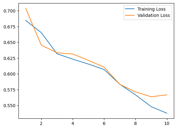
Acknowledgments#
Initial version: Mark Neubauer
Modified from the following Tutorial
© Copyright 2026