Reinforcement Learning#
Overview#
This technique is different than many of the other machine learning techniques we have seen earlier and has many applications in training agents (an AI) to interact with enviornments like games. Rather than feeding our machine learning model millions of examples we let our model come up with its own examples by exploring an enviornemt. The concept is simple. Humans learn by exploring and learning from mistakes and past experiences so let’s have our computer do the same.
Reinforcement learning methods are used for sequential decision making in uncertain environments. It is typically framed as an agent (the learner) interacting with an environment which provides the agent with reinforcement (positive or negative), based on the agent’s decisions. The agent leverages this reinforcement to update its behaviour in an aim to get closer to acting optimally. In interacting with the uncertain environment, the agent is also learning about the dynamics of the underlying system.
Terminology#
Before we dive into explaining reinforcement learning we need to define a few key peices of terminology.
Environment: In reinforcement learning tasks we have a notion of the enviornment. This is what our agent will explore. An example of an enviornment in the case of training an AI to play say a game of mario would be the level we are training the agent on.
Agent: an agent is an entity that is exploring the enviornment. Our agent will interact and take different actions within the enviornment. In our mario example the mario character within the game would be our agent.
State: always our agent will be in what we call a state. The state simply tells us about the status of the agent. The most common example of a state is the location of the agent within the enviornment. Moving locations would change the agents state.
Actions: any interaction between the agent and enviornment would be considered an action. For example, moving to the left or jumping would be an action. An action may or may not change the current state of the agent. In fact, the act of doing nothing is an action as well! The action of say not pressing a key if we are using our mario example.
Reward: every action that our agent takes will result in a reward of some magnitude (positive or negative). The goal of our agent will be to maximize its reward in an enviornment. Sometimes the reward will be clear, for example if an agent performs an action which increases their score in the enviornment we could say they’ve recieved a positive reward. If the agent were to perform an action which results in them losing score or possibly dying in the enviornment then they would recieve a negative reward.
The most important part of reinforcement learning is determing how to reward the agent. After all, the goal of the agent is to maximize its rewards. This means we should reward the agent appropiatly such that it reaches the desired goal.
Typical RL Flow#
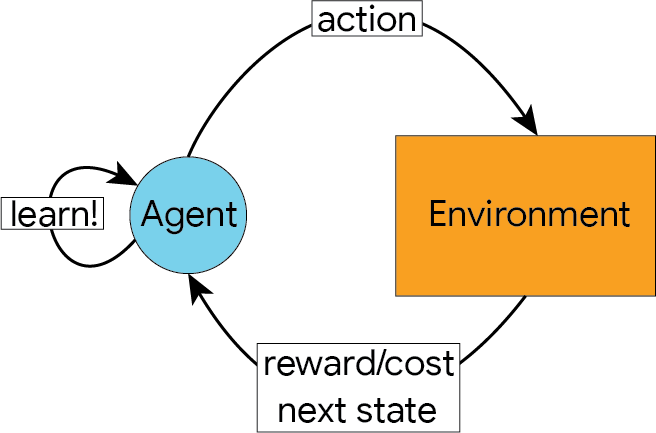
The following image depicts the typical flow of a reinforcement learning problem.
An agent, at some state in the environment, sends an action to the environment
The environment responds by providing the agent with:
A reward/cost that depends on the state the agent was in and the action chosen
A new state that the agent transitions to after performing the selected action (which can sometimes be the same state the agent was already in).
The agent then uses this information to update its behaviour so that it increases the likelihood of choosing actions that give a positive reward, and reduces the likelihood of choosing actions that result in a penalty.
Deep Q-Learning Network (DQN) Example #
This example shows how to use PyTorch to train a Deep Q Learning (DQN) agent on the CartPole-v1 task from Gymnasium.
Task#
The agent has to decide between two actions - moving the cart left or right - so that the pole attached to it stays upright. You can find more information about the environment and other more challenging environments at Gymnasium’s website.

As the agent observes the current state of the environment and chooses an action, the environment transitions to a new state, and also returns a reward that indicates the consequences of the action. In this task, rewards are +1 for every incremental timestep and the environment terminates if the pole falls over too far or the cart moves more than 2.4 units away from center. This means better performing scenarios will run for longer duration, accumulating larger return.
The CartPole task is designed so that the inputs to the agent are 4 real values representing the environment state (position, velocity, etc.). We take these 4 inputs without any scaling and pass them through a small fully-connected network with 2 outputs, one for each action. The network is trained to predict the expected value for each action, given the input state. The action with the highest expected value is then chosen.
Packages#
First, let’s import needed packages. Firstly, we need gymnasium for the environment, installed by using [pip]{.title-ref}. This is a fork of the original OpenAI Gym project and maintained by the same team since Gym v0.19. If you are running this in Google Colab, run:
%%bash
pip3 install gymnasium[classic_control]
We’ll also use the following from PyTorch:
neural networks (
torch.nn)optimization (
torch.optim)automatic differentiation (
torch.autograd)
DQN for CartPole Implementation#
!pip3 install gymnasium[classic_control]
Collecting gymnasium[classic_control]
  Downloading gymnasium-0.29.1-py3-none-any.whl (953 kB)
     ━━━━━━━━━━━━━━━━━━━━━━━━━━━━━━━━━━━━━━━━ 953.9/953.9 kB 4.6 MB/s eta 0:00:00
?25hRequirement already satisfied: numpy>=1.21.0 in /usr/local/lib/python3.10/dist-packages (from gymnasium[classic_control]) (1.25.2)
Requirement already satisfied: cloudpickle>=1.2.0 in /usr/local/lib/python3.10/dist-packages (from gymnasium[classic_control]) (2.2.1)
Requirement already satisfied: typing-extensions>=4.3.0 in /usr/local/lib/python3.10/dist-packages (from gymnasium[classic_control]) (4.10.0)
Collecting farama-notifications>=0.0.1 (from gymnasium[classic_control])
  Downloading Farama_Notifications-0.0.4-py3-none-any.whl (2.5 kB)
Requirement already satisfied: pygame>=2.1.3 in /usr/local/lib/python3.10/dist-packages (from gymnasium[classic_control]) (2.5.2)
Installing collected packages: farama-notifications, gymnasium
Successfully installed farama-notifications-0.0.4 gymnasium-0.29.1
%matplotlib inline
import gymnasium as gym
import math
import random
import matplotlib
import matplotlib.pyplot as plt
from collections import namedtuple, deque
from itertools import count

import torch
import torch.nn as nn
import torch.optim as optim
import torch.nn.functional as F

env = gym.make("CartPole-v1")

# set up matplotlib
is_ipython = 'inline' in matplotlib.get_backend()
if is_ipython:
    from IPython import display

plt.ion()

# if GPU is to be used
device = torch.device("cuda" if torch.cuda.is_available() else "cpu")
Replay Memory#
We’ll be using experience replay memory for training our DQN. It stores the transitions that the agent observes, allowing us to reuse this data later. By sampling from it randomly, the transitions that build up a batch are decorrelated. It has been shown that this greatly stabilizes and improves the DQN training procedure.
For this, we’re going to need two classes:
Transition- a named tuple representing a single transition in our environment. It essentially maps (state, action) pairs to their (next_state, reward) result, with the state being the screen difference image as described later on.ReplayMemory- a cyclic buffer of bounded size that holds the transitions observed recently. It also implements a.sample()method for selecting a random batch of transitions for training.
Transition = namedtuple('Transition',
                        ('state', 'action', 'next_state', 'reward'))


class ReplayMemory(object):

    def __init__(self, capacity):
        self.memory = deque([], maxlen=capacity)

    def push(self, *args):
        """Save a transition"""
        self.memory.append(Transition(*args))

    def sample(self, batch_size):
        return random.sample(self.memory, batch_size)

    def __len__(self):
        return len(self.memory)
DQN Algorithm#
Now, let’s define our model. But first, let’s quickly recap what a DQN is.
Our environment is deterministic, so all equations presented here are also formulated deterministically for the sake of simplicity. In the reinforcement learning literature, they would also contain expectations over stochastic transitions in the environment.
Our aim will be to train a policy that tries to maximize the discounted, cumulative reward \(R_{t_0} = \sum_{t=t_0}^{\infty} \gamma^{t - t_0} r_t\), where \(R_{t_0}\) is also known as the return. The discount, \(\gamma\), should be a constant between \(0\) and \(1\) that ensures the sum converges. A lower \(\gamma\) makes rewards from the uncertain far future less important for our agent than the ones in the near future that it can be fairly confident about. It also encourages agents to collect reward closer in time than equivalent rewards that are temporally far away in the future.
The main idea behind Q-learning is that if we had a function \(Q^*: State \times Action \rightarrow \mathbb{R}\), that could tell us what our return would be, if we were to take an action in a given state, then we could easily construct a policy that maximizes our rewards:
However, we don’t know everything about the world, so we don’t have access to \(Q^*\). But, since neural networks are universal function approximators, we can simply create one and train it to resemble \(Q^*\).
For our training update rule, we’ll use a fact that every \(Q\) function for some policy obeys the Bellman equation:
The Bellman equations states that the long-term reward in a given action is equal to the reward from the current action combined with the expected reward from the future actions taken at the following time.
The difference between the two sides of the equality is known as the temporal difference error, \(\delta\):
To minimize this error, we will use the Huber loss. The Huber loss acts like the mean squared error when the error is small, but like the mean absolute error when the error is large - this makes it more robust to outliers when the estimates of \(Q\) are very noisy. We calculate this over a batch of transitions, \(B\), sampled from the replay memory:
Q-Network#
Our model will be a feed forward neural network that takes in the difference between the current and previous screen patches. It has two outputs, representing \(Q(s, \mathrm{left})\) and \(Q(s, \mathrm{right})\) (where \(s\) is the input to the network). In effect, the network is trying to predict the expected return of taking each action given the current input.
class DQN(nn.Module):

    def __init__(self, n_observations, n_actions):
        super(DQN, self).__init__()
        self.layer1 = nn.Linear(n_observations, 128)
        self.layer2 = nn.Linear(128, 128)
        self.layer3 = nn.Linear(128, n_actions)

    # Called with either one element to determine next action, or a batch
    # during optimization. Returns tensor([[left0exp,right0exp]...]).
    def forward(self, x):
        x = F.relu(self.layer1(x))
        x = F.relu(self.layer2(x))
        return self.layer3(x)
Hyperparameters and Utilities#
This cell instantiates our model and its optimizer, and defines some utilities:
select_action- will select an action accordingly to an epsilon greedy policy. Simply put, we’ll sometimes use our model for choosing the action, and sometimes we’ll just sample one uniformly. The probability of choosing a random action will start atEPS_STARTand will decay exponentially towardsEPS_END.EPS_DECAYcontrols the rate of the decay.plot_durations- a helper for plotting the duration of episodes, along with an average over the last 100 episodes (the measure used in the official evaluations). The plot will be underneath the cell containing the main training loop, and will update after every episode.
# BATCH_SIZE is the number of transitions sampled from the replay buffer
# GAMMA is the discount factor as mentioned in the previous section
# EPS_START is the starting value of epsilon
# EPS_END is the final value of epsilon
# EPS_DECAY controls the rate of exponential decay of epsilon, higher means a slower decay
# TAU is the update rate of the target network
# LR is the learning rate of the ``AdamW`` optimizer
BATCH_SIZE = 128
GAMMA = 0.99
EPS_START = 0.9
EPS_END = 0.05
EPS_DECAY = 1000
TAU = 0.005
LR = 1e-4

# Get number of actions from gym action space
n_actions = env.action_space.n
# Get the number of state observations
state, info = env.reset()
n_observations = len(state)

policy_net = DQN(n_observations, n_actions).to(device)
target_net = DQN(n_observations, n_actions).to(device)
target_net.load_state_dict(policy_net.state_dict())

optimizer = optim.AdamW(policy_net.parameters(), lr=LR, amsgrad=True)
memory = ReplayMemory(10000)


steps_done = 0


def select_action(state):
    global steps_done
    sample = random.random()
    eps_threshold = EPS_END + (EPS_START - EPS_END) * \
        math.exp(-1. * steps_done / EPS_DECAY)
    steps_done += 1
    if sample > eps_threshold:
        with torch.no_grad():
            # t.max(1) will return the largest column value of each row.
            # second column on max result is index of where max element was
            # found, so we pick action with the larger expected reward.
            return policy_net(state).max(1).indices.view(1, 1)
    else:
        return torch.tensor([[env.action_space.sample()]], device=device, dtype=torch.long)


episode_durations = []


def plot_durations(show_result=False):
    plt.figure(1)
    durations_t = torch.tensor(episode_durations, dtype=torch.float)
    if show_result:
        plt.title('Result')
    else:
        plt.clf()
        plt.title('Training...')
    plt.xlabel('Episode')
    plt.ylabel('Duration')
    plt.plot(durations_t.numpy())
    # Take 100 episode averages and plot them too
    if len(durations_t) >= 100:
        means = durations_t.unfold(0, 100, 1).mean(1).view(-1)
        means = torch.cat((torch.zeros(99), means))
        plt.plot(means.numpy())

    plt.pause(0.001)  # pause a bit so that plots are updated
    if is_ipython:
        if not show_result:
            display.display(plt.gcf())
            display.clear_output(wait=True)
        else:
            display.display(plt.gcf())
Training Loop#
Finally, the code for training our model.
Here, you can find an optimize_model function that performs a single
step of the optimization. It first samples a batch, concatenates all the
tensors into a single one, computes \(Q(s_t, a_t)\) and
\(V(s_{t+1}) = \max_a Q(s_{t+1}, a)\), and combines them into our loss. By
definition we set \(V(s) = 0\) if \(s\) is a terminal state. We also use a
target network to compute \(V(s_{t+1})\) for added stability. The target
network is updated at every step with a soft
update controlled by the
hyperparameter TAU, which was previously defined.
def optimize_model():
    if len(memory) < BATCH_SIZE:
        return
    transitions = memory.sample(BATCH_SIZE)
    # Transpose the batch (see https://stackoverflow.com/a/19343/3343043 for
    # detailed explanation). This converts batch-array of Transitions
    # to Transition of batch-arrays.
    batch = Transition(*zip(*transitions))

    # Compute a mask of non-final states and concatenate the batch elements
    # (a final state would've been the one after which simulation ended)
    non_final_mask = torch.tensor(tuple(map(lambda s: s is not None,
                                          batch.next_state)), device=device, dtype=torch.bool)
    non_final_next_states = torch.cat([s for s in batch.next_state
                                                if s is not None])
    state_batch = torch.cat(batch.state)
    action_batch = torch.cat(batch.action)
    reward_batch = torch.cat(batch.reward)

    # Compute Q(s_t, a) - the model computes Q(s_t), then we select the
    # columns of actions taken. These are the actions which would've been taken
    # for each batch state according to policy_net
    state_action_values = policy_net(state_batch).gather(1, action_batch)

    # Compute V(s_{t+1}) for all next states.
    # Expected values of actions for non_final_next_states are computed based
    # on the "older" target_net; selecting their best reward with max(1).values
    # This is merged based on the mask, such that we'll have either the expected
    # state value or 0 in case the state was final.
    next_state_values = torch.zeros(BATCH_SIZE, device=device)
    with torch.no_grad():
        next_state_values[non_final_mask] = target_net(non_final_next_states).max(1).values
    # Compute the expected Q values
    expected_state_action_values = (next_state_values * GAMMA) + reward_batch

    # Compute Huber loss
    criterion = nn.SmoothL1Loss()
    loss = criterion(state_action_values, expected_state_action_values.unsqueeze(1))

    # Optimize the model
    optimizer.zero_grad()
    loss.backward()
    # In-place gradient clipping
    torch.nn.utils.clip_grad_value_(policy_net.parameters(), 100)
    optimizer.step()
Below, you can find the main training loop. At the beginning we reset
the environment and obtain the initial state Tensor. Then, we sample
an action, execute it, observe the next state and the reward (always 1),
and optimize our model once. When the episode ends (our model fails), we
restart the loop.
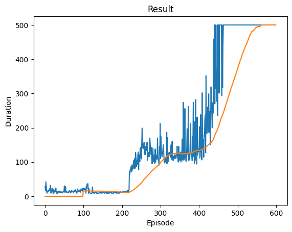
Below, [num_episodes]{.title-ref} is set to 600 if a GPU is available, otherwise 50 episodes are scheduled so training does not take too long. However, 50 episodes is insufficient for to observe good performance on CartPole. You should see the model constantly achieve 500 steps within 600 training episodes. Training RL agents can be a noisy process, so restarting training can produce better results if convergence is not observed.
if torch.cuda.is_available():
    num_episodes = 600
else:
    num_episodes = 50

for i_episode in range(num_episodes):
    # Initialize the environment and get its state
    state, info = env.reset()
    state = torch.tensor(state, dtype=torch.float32, device=device).unsqueeze(0)
    for t in count():
        action = select_action(state)
        observation, reward, terminated, truncated, _ = env.step(action.item())
        reward = torch.tensor([reward], device=device)
        done = terminated or truncated

        if terminated:
            next_state = None
        else:
            next_state = torch.tensor(observation, dtype=torch.float32, device=device).unsqueeze(0)

        # Store the transition in memory
        memory.push(state, action, next_state, reward)

        # Move to the next state
        state = next_state

        # Perform one step of the optimization (on the policy network)
        optimize_model()

        # Soft update of the target network's weights
        # θ′ ← τ θ + (1 −τ )θ′
        target_net_state_dict = target_net.state_dict()
        policy_net_state_dict = policy_net.state_dict()
        for key in policy_net_state_dict:
            target_net_state_dict[key] = policy_net_state_dict[key]*TAU + target_net_state_dict[key]*(1-TAU)
        target_net.load_state_dict(target_net_state_dict)

        if done:
            episode_durations.append(t + 1)
            plot_durations()
            break

print('Complete')
plot_durations(show_result=True)
plt.ioff()
plt.show()
Complete
<Figure size 640x480 with 0 Axes>
<Figure size 640x480 with 0 Axes>
Here is the diagram that illustrates the overall resulting data flow.
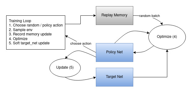
Actions are chosen either randomly or based on a policy, getting the next step sample from the gym environment. We record the results in the replay memory and also run optimization step on every iteration. Optimization picks a random batch from the replay memory to do training of the new policy. The “older” target_net is also used in optimization to compute the expected Q values. A soft update of its weights are performed at every step.
Acknowledgments#
Initial version: Mark Neubauer
Author: Adam Paszke
From this notebook
© Copyright 2026