Supervised Learning#
%matplotlib inline
import matplotlib.pyplot as plt
import seaborn as sns; sns.set_theme()
import numpy as np
import pandas as pd
import os.path
import subprocess
import scipy.linalg
from sklearn import linear_model
import warnings
warnings.filterwarnings('ignore')
Helpers for Getting, Loading and Locating Data
def wget_data(url: str):
    local_path = './tmp_data'
    p = subprocess.Popen(["wget", "-nc", "-P", local_path, url], stderr=subprocess.PIPE, encoding='UTF-8')
    rc = None
    while rc is None:
      line = p.stderr.readline().strip('\n')
      if len(line) > 0:
        print(line)
      rc = p.poll()

def locate_data(name, check_exists=True):
    local_path='./tmp_data'
    path = os.path.join(local_path, name)
    if check_exists and not os.path.exists(path):
        raise RuxntimeError('No such data file: {}'.format(path))
    return path
Get Data#
wget_data('https://raw.githubusercontent.com/illinois-mlp/MachineLearningForPhysics/main/data/line_data.csv')
wget_data('https://raw.githubusercontent.com/illinois-mlp/MachineLearningForPhysics/main/data/line_targets.csv')
File ‘./tmp_data/line_data.csv’ already there; not retrieving.
--2026-02-16 20:45:38--  https://raw.githubusercontent.com/illinois-mlp/MachineLearningForPhysics/main/data/line_targets.csv
Resolving raw.githubusercontent.com (raw.githubusercontent.com)... 185.199.110.133, 185.199.111.133, 185.199.108.133, ...
Connecting to raw.githubusercontent.com (raw.githubusercontent.com)|185.199.110.133|:443... connected.
HTTP request sent, awaiting response... 200 OK
Length: 39419 (38K) [text/plain]
Saving to: ‘./tmp_data/line_targets.csv’
     0K .......... .......... .......... ........             100% 3.48M=0.01s
2026-02-16 20:45:38 (3.48 MB/s) - ‘./tmp_data/line_targets.csv’ saved [39419/39419]
Load Data#
line_data    = pd.read_csv(locate_data('line_data.csv'))
line_targets = pd.read_csv(locate_data('line_targets.csv'))
Supervised Learning in Scikit Learn#
The sklearn supervised learning functions are organized into several modules:
linear_model: regression with generalized linear models.
kernel_ridge: ridge regression using the kernel trick.
svm: regression, classification (and outlier detection) with support vector machines.
tree: regression and classification using decision trees.
discriminant_analysis: classification using linear and quadratic discriminant analysis.
ensemble: regression, classification (and anomaly detection) using ensemble methods.
gaussian_process: regression and classification using Gaussian processes.
naive_bayes: Bayesian classification with oversimplified assumptions.
More esoteric and less used supervised learning modules:
isotonic: regression using an isotonic model.
multiclass and multioutput: meta-estimators that enhance a base estimator.
neural_network: we will use tensorflow instead to implement neural networks algorithms.
Finally, useful infrastructure for supervised learning:
preprocessing: prepare your data before learning from it.
pipeline: utilities to chain together estimators (and preprocessing) into a single pipeline.
model_selection: model selection (hyper-parameter tuning) via cross validation.
Since regression problems are more common in scientific applications, we will focus on them here. Our earlier introduction of supervised learning used a probabilistic language where the solution is given by a distribution
Stated differently, our goal is, given a training set of random variables \(X\) and \(Y\) (i.e. \(D\)), to learn a function
so that \(h(x)\) is a “good” predictor for the corresponding value of \(y\). For historical reasons, this function \(h(x)\) is called a hypothesis.
When the target variable that we are trying to predict is continuous, we call the learning problem a regression problem. When \(Y\) can take on only a small number of discrete values, we call it a classification problem.
Unfortunately, most sklearn algorithms give only limited information about this distribution, since they only return an estimate of its central tendency (mean / median / mode / …):
In practice, if you need to make probabilistic statements about what you have learned from a regression, your best choices among the sklearn algorithms are:
Linear regression to model (approximately) linear relationships.
Gaussian process regression to model non-linear relationships.
Linear Regression#
Ordinary linear regression predicts the expected value of a given unknown quantity (the response variable, a random variable) as a linear combination of a set of observed values (predictors). This implies that a constant change in a predictor leads to a constant change in the response variable (i.e. a linear-response model).
A standard linear regression assumes the observed data \(D = (X,Y)\) is explained by the model,
where, in general, all quantities are matrices, the model parameters are the elements of \(W\), and \(\delta Y\) is the “noise” inherent in \(Y\).
EXERCISE: Assume that \(X\) consists of \(N\) samples of \(n\) features, represented by a \(N\times n\) matrix, and \(Y\) consists of \(N\) samples of \(m\) features, represented by a \(N\times m\) matrix. What are the dimensions of the matrices for \(W\) and \(\delta Y\)?
\(W\) must be \(n\times m\), in order that the matrix product \(X W\) has the shape \(N\times m\).
\(\delta Y\) must have the same shape as \(Y\): \(N\times m\).
When \(m=1\), the linear regression problem is usually written with lower-case notation:
We further assume that:
There is no (or negligible) noise in \(X\).
Each feature in \(Y\) has zero mean, i.e.,
np.mean(Y, axis=0) = 0.
If the last condition is not met, we could simply subtract the mean before applying this model,
Y -= np.mean(Y, axis=0)
but we will see that sklearn will do this automatically for you.
By definition, “noise” is unbiased,
and uncorrelated with \(X\),
The noise is usually assumed to be Gaussian but, in the most general case, this is complex to model since there are potentially \(n^2 m^2\) covariances (only ~half of which are independent),
to account for:
different variances for each of the \(m\) features in \(Y\), and
correlations between the \(m\) features in \(Y\), and
correlations between the \(N\) samples in \(Y\).
In practice, the most general problem we solve is when
i.e., all \(m\) features have the same variance \(C_{ii}\) for sample \(i\), but samples are potentially correlated. The resulting \(n\times n\) “sample covariance matrix” \(C\) then specifies the likelihood
where \((Y - X W)_k\) is the column of \(N\) values (one per sample) for the \(k\)-th feature of \(Y\). Note that we treat the elements of \(C\) as fixed hyperparameters in standard linear regression.
A important special case occurs when all samples (and features) have the same variance \(\sigma^2\),
which we refer to as homoscedastic errors. Any type of non-homescedastic errors are called heteroscedastic.
Example: Fitting a Line#
Read our line_data dataset:
D = line_data
X = D['x'].values.reshape(-1, 1)
y = D['y'].values
y_true = line_targets['y_true'].values
The LinearRegression function solves the linear least squares problem by minimizing sum of squared residuals
with respect to the model parameters (elements of \(W\)), where \(i\) indexes the \(N\) samples in the dataset. The syntax will be familiar from the sklearn functions we used earlier:
fit = linear_model.LinearRegression(fit_intercept=True).fit(X, y)
Note that LinearRegression will automatically calculate and subtract any non-zero mean of \(y\) when fit_intercept is True.
The resulting \(W\) matrix has only a single element, the slope of the line (which is assumed to pass through the origin):
W = fit.coef_
y0 = fit.intercept_
plt.scatter(X[:, 0], y, label='D=(X,y)', lw=0, s=5, c='gray')
plt.plot(X[:, 0], X.dot(W) + y0, 'r-', lw=8, alpha=0.5, label='fit')
plt.plot(X[:, 0], y_true, 'k-', label='truth')
plt.legend(fontsize='x-large')
plt.xlabel('$X$')
plt.ylabel('$y$')
plt.xlim(-1., +1.)
(-1.0, 1.0)
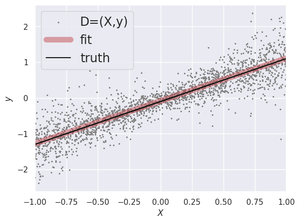
In our probabilistic language, LinearRegression finds the maximum likelihood (ML) point estimate assuming homoscedastic Gaussian errors. This can also be interpreted as a maximum a-posteriori (MAP) point estimate if we believe that the priors should all be uniform.
This ML solution can be found directly using linear algebra (which makes linear regression a very special case of supervised learning):
Note that the solution does not depend on the homoscedastic error \(\sigma\).
EXERCISE: Explain why we cannot simplify this expression using:
This is only valid when \(X\) is a square matrix, \(N = n\), in which case finding \(W\) reduces to solving a system of \(N\) linear equations in \(N\) unknowns. In the more general case where \(N > n\), we have an overdetermined system of equations and seek the best compromise solution given the expected errors. If \(N < n\), the problem is underdetermined and \(X^T X\) is not invertible.
We can also directly solve the more general problem of Gaussian errors described by an \(n\times n\) sample covariance \(C\):
However, the LinearRegression function can only solve the case where \(C\) is diagonal, i.e., each sample has a different variance but samples are uncorrelated:
Dvalid = D.dropna()
X = Dvalid['x'].values.reshape(-1, 1)
y = Dvalid['y'].values
dy = Dvalid['dy'].values
Pass the diagonal elements of \(C\) as the third argument to the fit method:
fit_w = linear_model.LinearRegression().fit(X, y, sample_weight=1 / (dy ** 2))
W_w = fit_w.coef_
y0_w = fit_w.intercept_
The weighted fit finds a slightly different solution since we are now giving more weight to observations near \(x = 0\) where \(\sigma^2\) is smaller.
print(np.round([W, W_w], 3))
[[1.194]
 [1.193]]
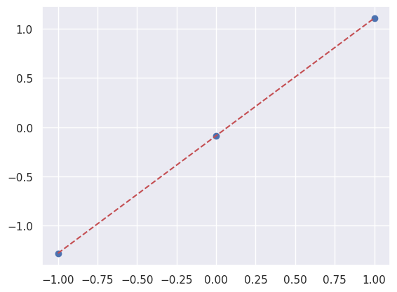
A LinearRegression fit can apply what is has learned to predict new data:
X_new = np.array([[-1], [0], [+1]])
y_new = fit_w.predict(X_new)
Not surprisingly, the predicted \(y\) values lie on the straight-line fit:
slope = W_w[0]
plt.scatter(X_new[:, 0], y_new);
plt.plot([-1, +1], [y0-slope, y0+slope], 'r--');
These are mean point estimates of \(Y'\) given new \(X'\), so of limited use when you want to make probabilistic statements about what your have learned. However, the likelihood is Gaussian in the model parameters:
where \(W_0\) is the ML weight matrix, \((W - W_0)_k\) is the \(k\)-th column with \(n\) rows, and \(E\) is its \(n\times n\) covariance, given by:
For homoscedastic errors \(\sigma\), this reduces to
Unfortunately, the LinearRegression fit does not calculate these errors for you, but they are straightforward to calculate yourself, for example:
C = np.diag(dy ** 2)
C_inv = np.diag(1 / (dy ** 2))
E = np.linalg.inv(np.dot(X.T, np.dot(C_inv, X)))
In this simple example, E is a \(1 \times 1\) matrix containing the variance of the slope:
dslope = np.sqrt(E[0,0])
plt.scatter(X_new[:, 0], y_new);
plt.fill_between([-1, +1], [y0-slope+dslope, y0+slope-dslope],
                 [y0-slope-dslope, y0+slope+dslope], color='r', alpha=0.5)
plt.xlabel('$X$')
plt.ylabel('$y$');
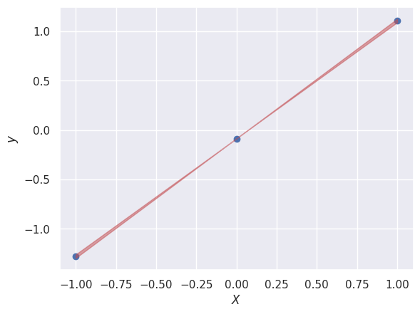
Note that we are not propagating the uncertainty in \(y_0\) here.
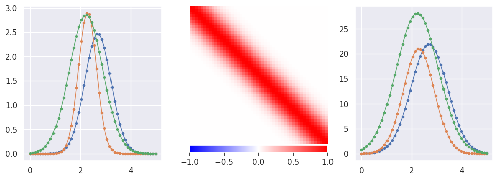
Example: Linear Deconvolution#
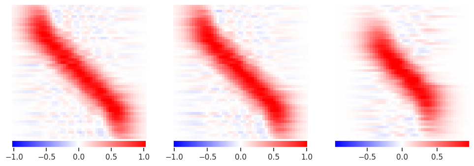
The examples above have a large \(N\) but only one feature in \(X\) and \(Y\), \(n=m=1\), so that \(W\) is just a single number, the slope of the line. For a more complex example, suppose we have an instrument with an unknown response, \(R(t,t')\), that transforms each input pulse \(z(t)\) into an output pulse via convolution
If we discretize time, \(t_k = k \Delta t\), then the corresponding discrete response model is linear:
with \(R_{ij} = R(t_i - t_j)\).
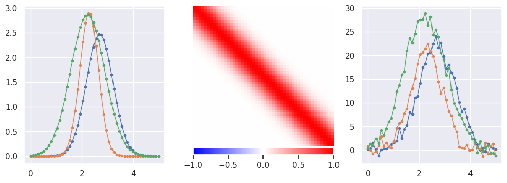
Generate some pulse data with a smooth Gaussian response:
def plot_response(R, ax):
    lim = np.percentile(np.abs(R), 99)
    img = ax.imshow(R, interpolation='none', cmap='bwr', vmin=-lim, vmax=+lim)
    plt.colorbar(img, ax=ax, orientation='horizontal', pad=0.01, fraction=0.1)
    ax.axis('off')
def generate(N=5000, n=50, tlo=0, thi=5, nplot=3, sigma_y = 0., seed=123):
    gen = np.random.RandomState(seed=seed)
    t_range = thi - tlo
    t0 = gen.uniform(tlo + 0.4 * t_range, thi - 0.4 * t_range, size=(N, 1))
    sigma = gen.uniform(0.05 * t_range, 0.15 * t_range, size=(N, 1))
    y0 = 1 + gen.rayleigh(size = (N, 1))
    t_grid = np.linspace(tlo, thi, n)
    X = y0 * np.exp(-0.5 * (t_grid - t0) ** 2 / sigma ** 2)
    r = np.exp(-0.5 * t_grid ** 2 / (t_range / 10) ** 2)
    R = scipy.linalg.toeplitz(r)
    Y = X.dot(R)
    Y += gen.normal(scale=sigma_y, size=Y.shape)
    fig, ax = plt.subplots(1, 3, figsize=(12, 4))
    for i in range(nplot):
        ax[0].plot(t_grid, X[i], '.-', lw=1)
        ax[2].plot(t_grid, Y[i], '.-', lw=1)
    plot_response(R, ax[1])
    return X, Y

X, Y = generate()
EXERCISE: With \(n\) features (timesteps) in the input data \(X\) and the same number \(m=n\) of features in the target data \(Y\), what is the minimum number of samples required to estimate the instrument response matrix \(R\)?
The response matrix has \(n m = n^2\) unknown parameters. While there are symmetries in \(R\) that could reduce this number significantly, a linear regression does not know about these symmetries.
Each of the \(N\) samples provides an independent linear equation in the unknown parameters. Therefore, the problem has an exact solution when \(N = n^2\) in the absence of any noise. When \(N < n^2\), the problem is formally ill-determined since \(X^T X\) is not invertible. However, a solution is still possible using a pseudo matrix inverse and sometimes gives reasonable results.
With \(N > n^2\), the problem is overdetermined, but we could expect additional samples to improve the answer when noise is present.
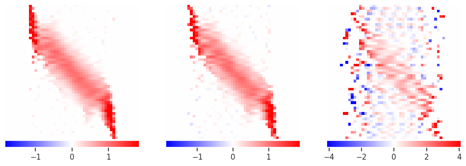
Try fitting with \(N = 2 n^2\), \(N = n^2\) or \(N = n\):
n = X.shape[1]
fit1 = linear_model.LinearRegression(fit_intercept=False).fit(X, Y)
fit2 = linear_model.LinearRegression(fit_intercept=False).fit(X[:n**2], Y[:n**2])
fit3 = linear_model.LinearRegression(fit_intercept=False).fit(X[:n], Y[:n])
R1, R2, R3 = fit1.coef_, fit2.coef_, fit3.coef_
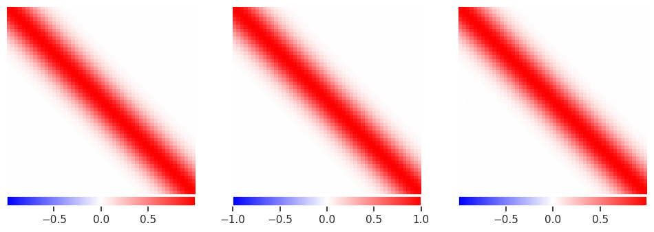
The results look reasonable in all cases, although there are some artifacts visible in the underdetermined solution:
def plot_responses(*Rlist):
    n = len(Rlist)
    fig, ax = plt.subplots(1, n, figsize=(4 * n, 4))
    for i, R in enumerate(Rlist):
        plot_response(R, ax[i])

plot_responses(R1, R2, R3)
The examples above have no noise in \(Y\) (except for tiny round-off errors) so now try adding some noise:
X, Y = generate(sigma_y=1)
fit1 = linear_model.LinearRegression(fit_intercept=False).fit(X, Y)
fit2 = linear_model.LinearRegression(fit_intercept=False).fit(X[:n**2], Y[:n**2])
fit3 = linear_model.LinearRegression(fit_intercept=False).fit(X[:n], Y[:n])
R1, R2, R3 = fit1.coef_, fit2.coef_, fit3.coef_
plot_responses(R1, R2, R3)
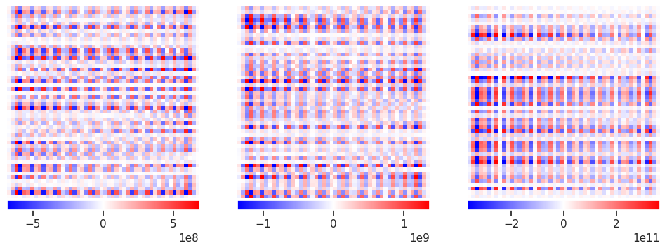
This clearly not what we are looking for, so what happened? The problem is that the solution amplifies noise and finds a “best” solution that involves large cancellations between positive (red) and negative (blue) values (notice the \(10^{12}\) in the colorbar scale!) This is not a problem that more samples can easily cure.
However, the true response is still a near-optimal solution but just very unlikely to be the most optimum solution when noise is present. In a Bayesian framework, this is when we would introduce a prior for our belief that a valid solution should be “smooth” and not require these large cancellations. Classical regression methods (and sklearn) refer to these priors as “regularization terms”, but they amount to the same thing.
Regularization is implemented as a penalty term \(R\) that we add to the least-squares score \(S\) defined above:
The most common approach is to penalize using
which goes by several names including Tikhanov regularization and ridge regression. Note that this introduces a hyperparameter \(\alpha\) which controls the strength of the regularization (prior) relative to the optimal solution (likelihood):
alpha = 0.1
fit1 = linear_model.Ridge(fit_intercept=False, alpha=alpha).fit(X, Y)
fit2 = linear_model.Ridge(fit_intercept=False, alpha=alpha).fit(X[:n**2], Y[:n**2])
fit3 = linear_model.Ridge(fit_intercept=False, alpha=alpha).fit(X[:n], Y[:n])
R1, R2, R3 = fit1.coef_, fit2.coef_, fit3.coef_
plot_responses(R1, R2, R3)
This has eliminated the wild fluctuations around \(\pm 10^{12}\) but is still noisy. Note how additional data now improves the solution, especially in the corners.
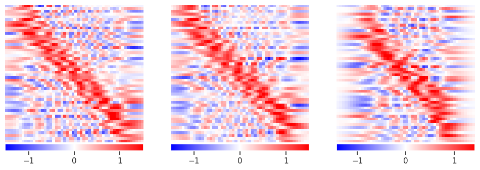
Try again with stronger regularization (priors):
alpha = 10.
fit1 = linear_model.Ridge(fit_intercept=False, alpha=alpha).fit(X, Y)
fit2 = linear_model.Ridge(fit_intercept=False, alpha=alpha).fit(X[:n**2], Y[:n**2])
fit3 = linear_model.Ridge(fit_intercept=False, alpha=alpha).fit(X[:n], Y[:n])
R1, R2, R3 = fit1.coef_, fit2.coef_, fit3.coef_
plot_responses(R1, R2, R3)
The sum of squares used in \(S\) and \(R\) above is called an L2 norm and measures the usual Euclidean distance:
Other norms are possible but generally more difficult to work with. The L0 norm is particularly interesting because it simply counts the number of non-zero elements in \(W\) so directly measures how sparse the solution is. The L1 norm,
is almost as good for measuring sparsity and much easier to optimize over than the L0 norm. (There has been a lot of recent interest in L0 and L1 norms in the context of compressed sensing.)
The “lasso” regression algorithm uses an L1 regularization term:
and is also implemented in sklearn (but noticeably slower):
alpha = 0.001
fit1 = linear_model.Lasso(fit_intercept=False, alpha=alpha).fit(X, Y)
fit2 = linear_model.Lasso(fit_intercept=False, alpha=alpha).fit(X[:n**2], Y[:n**2])
fit3 = linear_model.Lasso(fit_intercept=False, alpha=alpha).fit(X[:n], Y[:n])
R1, R2, R3 = fit1.coef_, fit2.coef_, fit3.coef_
plot_responses(R1, R2, R3)
The results are indeed sparse, but that is probably not the best prior to use in this problem.
For more regularization options, look at ElasticNet which combines both L2 and L1 terms.
Example: Basis Function Linear Regression#
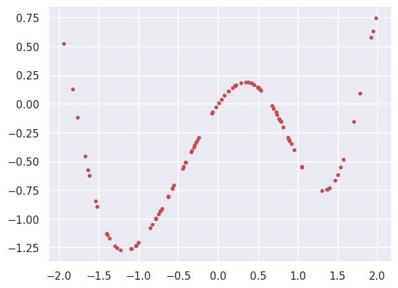
For our final example, we will see how “linear” regression can solve problems that appear quite nonlinear. Suppose our model is
with unknown parameters \(a\) and \(b\):
def generate(N=100, xlo=-2, xhi=2, a=1, b=-1, seed=123):
    gen = np.random.RandomState(seed=seed)
    X = gen.uniform(xlo, xhi, N)
    y = a * X * np.exp(-X ** 2) + b * np.sin(X ** 2)
    plt.plot(X, y, 'r.')
    return X, y

X, y = generate()
If we replace the \(N\times 1\) dataset \(X\) with a \(N\times 2\) dataset \(Z\) of new features \((Z_1, Z_2)\):
the transformed model is now linear:
with
The new features \(Z_1\) and \(Z_2\) are known as basis functions and this approach is called basis function regression. Sklearn has built-in support for polynomial basis functions but it is easy to apply the transformations yourself for arbitrary basis functions:
Z = np.stack([X * np.exp(-X ** 2), np.sin(X ** 2)], axis=1)
Z.shape
(100, 2)
fit = linear_model.LinearRegression(fit_intercept=False).fit(Z, y)
print(fit.coef_)
[ 1. -1.]
DISCUSS: Suppose we have a multiplicative model for our data,
would it be valid to transform \(y \rightarrow \log y\) and treat this as a linear regression problem?
Since
we could use
and solve for \(a\) and \(b\) as linear-regression coefficients. This is a useful trick, but with an important caveat: the linear regression solution assumes Gaussian uncertainties in \(y\), but after this transform you would need Gaussian uncertainties in \(\log y\). In particular, if your original uncertainties in \(y\) were Gaussian, they will not be Gaussian in \(\log y\).
Note that the uncertainties are not an issue when we only transform \(X\) since we assume \(X\) is noise free.
Acknowledgments#
Initial version: Mark Neubauer
© Copyright 2026