Jupyter Notebooks and Numerical Python

Jupyter Notebooks and Numerical Python#

Jupyter Notebooks#

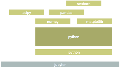
Jupyter is an interactive front-end to a rich ecosystem of python packages that support machine learning and data science tasks. We will use the core set of packages shown below for this course:

All course notebooks begin with some preamble code to import and configure some frequently used packages:

%matplotlib inline
import matplotlib.pyplot as plt
import seaborn as sns; sns.set()
import numpy as np
import pandas as pd

You might see a warning about “building the font cache” if this is your first time using the course conda environment, but any other message probably indicates that you do not have your environment set up correctly yet.

Here are the actual package versions we are using:

import matplotlib
print('matplotlib', matplotlib.__version__)
print('seaborn', sns.__version__)
print('numpy', np.__version__)
print('pandas', pd.__version__)

matplotlib 3.7.0
seaborn 0.12.2
numpy 1.23.5
pandas 2.0.3

You will get plenty of experience with notebooks during this course so we will start with just a few basic survival skills. For a deeper dive, start with IPython: Beyond Normal Python in the Python Data Science Handbook.

Type command? to display help on command. Try this now for the built-in range function then dismiss the help window.

Hit the tab key to display possible completions of a partial name. Try this now by typing np.arc below then hitting TAB.

Your notebook will sometimes be unresponsive while executing a long command that you don’t want to wait for. Use the Interrupt command in the Kernel menu to recover from situations like this. Try this out now by:

Uncomment the time.sleep(3600) line below, which sleeps for an hour.
Execute the cell and note the In [*] to the left while it is running.
Interrupt the kernel.

import time
#time.sleep(3600)

In more extreme cases you may need to use the Restart command, which puts your kernel in a well-defined initial state (good) but also forgets any variables or functions you have already defined (bad). Try this now by:

Re-running the sleep cell above.
Restarting the kernel. Note that this leaves [*] next to the cell, which is misleading.
Comment out the time.sleep(3600) line above.
Rebuild the kernel state using Run All Above from the Cell menu. This fixes the [*].

Numerical Python#

This section introduces the “numpy” package. For further reading, see Introduction to NumPy in the Python Data Science Handbook.

Rationale#

The problem that numpy addresses is that python lists are very flexible, but not optimized for the special case where all list elements are numeric values of the same type, which can be very efficiently organized in memory. Numpy provides a specialized array with lots of nice features. One downside of this approach is that most of builtin math functions are duplicated (e.g., math.sin and np.sin) to work with numpy arrays.

In this example, we fill a list with values \(\sin(\pi k / n)\) using plain python and the builtin math package (if the use of spaces in math.pi * k / n looks odd, see PEP8):

import math

def create_python_array(n=100):
    x = []
    for k in range(n):
        x.append(math.sin(math.pi * k / n))
    return x

Use an ipython magic command to time this function for a large array:

%time x1 = create_python_array(1000000)

CPU times: user 107 ms, sys: 8.67 ms, total: 116 ms
Wall time: 115 ms

The resulting list is very flexible so, for example, we can replace any value with a completely different type or append new values:

x1[3] = 'not a number'
x1.append(-1)

The corresponding python code uses numpy functions and does not require any python loop (which is often a bottleneck):

def create_numpy_array(n=100):
    k = np.arange(n)
    x = np.sin(np.pi * k / n)
    return x

%time x2 = create_numpy_array(1000000)

CPU times: user 8.38 ms, sys: 4.08 ms, total: 12.5 ms
Wall time: 12.1 ms

The resulting numpy array holds only 64-bit floating point numbers and has a fixed size:

try:
    x2[2] = 'not a number'
except ValueError as e:
    print(e)

could not convert string to float: 'not a number'

Create Arrays#

The most common ways you will create arrays are:

Filled with a regular sequence of values.
Filled with random values.
Calculated as a mathematical function of other arrays.

The exercises below will give you some practice, with pointers to the numpy functions to use (Use the builtin notebook help to learn more about them).

EXAMPLE: Use np.arange to create an array of integers 0, 1, …, 9:

np.arange(10)

array([0, 1, 2, 3, 4, 5, 6, 7, 8, 9])

EXAMPLE: Use np.linspace to create an array of 11 floats 0.0, 0.1, …, 0.9, 1.0:

np.linspace(0., 1., 11)

array([0. , 0.1, 0.2, 0.3, 0.4, 0.5, 0.6, 0.7, 0.8, 0.9, 1. ])

EXAMPLE: Use np.random.RandomState to initialize a reproducible (pseudo)random number generator using the seed 123:

generator = np.random.RandomState(seed=123)

EXAMPLE: Use np.random.uniform to generate an array of 10 uniformly distributed random numbers in the interval [0,1]:

generator.uniform(size=10)

array([0.69646919, 0.28613933, 0.22685145, 0.55131477, 0.71946897,
       0.42310646, 0.9807642 , 0.68482974, 0.4809319 , 0.39211752])

EXAMPLE: Use np.random.normal to generate an array of 10 random numbers drawn from a normal (aka Gaussian) distribution with mean -1 and standard deviation 2:

generator.normal(loc=-1, scale=2, size=10)

array([ 1.53187252, -2.7334808 , -2.3577723 , -1.18941794,  1.98277925,
       -2.27780399, -1.88796392, -1.86870255,  3.41186017,  3.37357218])

EXAMPLE: Generate arrays x, y, z of length 10 with values drawn from a “unit” Gaussian distribution (mean=0, std=1):

x = generator.normal(size=10)
y = generator.normal(size=10)
z = generator.normal(size=10)

EXAMPLE: Adjust the values in x, y, z so that the vectors (x,y,z) are normalized. (This is a useful trick for generating random points that are uniformly distributed on a unit sphere).

r = np.sqrt(x ** 2 + y ** 2 + z ** 2)
x /= r
y /= r
z /= r

EXAMPLE: Calculate arrays theta and phi containing the polar angles in degrees for each vector (x, y, z). Use np.arccos, np.arctan2, np.degrees.

theta = np.degrees(np.arccos(z))
phi = np.degrees(np.arctan2(y, x))

Multidimensional Arrays#

The examples above all create 1D arrays, but numpy arrays can have multiple dimensions (aka “shapes”):

vector = np.ones(shape=(4,))
matrix = np.ones(shape=(3, 4))
tensor = np.ones(shape=(2, 3, 4))

Access array elements with zero-based indexing:

vector[1] # single element

1.0

matrix[1, :] # single row

array([1., 1., 1., 1.])

matrix[:, 1] # single column

array([1., 1., 1.])

tensor[0, :2, :2] # submatrix

array([[1., 1.],
       [1., 1.]])

Use np.dot to calculate inner products:

vector.dot(vector)

4.0

matrix.dot(vector)

array([4., 4., 4.])

Arrays of the same shape can be combined in “vectorized” operations (i.e., without any explicit loops):

matrix + np.sin(matrix ** 2)

array([[1.84147098, 1.84147098, 1.84147098, 1.84147098],
       [1.84147098, 1.84147098, 1.84147098, 1.84147098],
       [1.84147098, 1.84147098, 1.84147098, 1.84147098]])

Arrays of different shapes can also be combined when they are compatible according to the broadcasting rules. Note that the broadcasting rules do not depend on the operations being used so, for example, if x + y is valid, then so is x * y ** 2 + x ** 2 * y.

matrix + 0.1

array([[1.1, 1.1, 1.1, 1.1],
       [1.1, 1.1, 1.1, 1.1],
       [1.1, 1.1, 1.1, 1.1]])

vector + matrix

array([[2., 2., 2., 2.],
       [2., 2., 2., 2.],
       [2., 2., 2., 2.]])

Define a function to try broadcasting two arbitrary shapes:

def broadcast(shape1, shape2):
    array1 = np.ones(shape1)
    array2 = np.ones(shape2)
    try:
        array12 = array1 + array2
        print('shapes {} {} broadcast to {}'.format(shape1, shape2, array12.shape))
    except ValueError as e:
        print(e)

broadcast((1, 3), (3,))

shapes (1, 3) (3,) broadcast to (1, 3)

broadcast((1, 2), (3,))

operands could not be broadcast together with shapes (1,2) (3,)

EXERCISE: Predict the results of the following:

broadcast((3, 1, 2), (3, 2))
broadcast((2, 1, 3), (3, 2))
broadcast((3,), (2, 1))
broadcast((3,), (1, 2))
broadcast((3,), (1, 3))

broadcast((3, 1, 2), (3, 2))
broadcast((2, 1, 3), (3, 2))
broadcast((3,), (2, 1))
broadcast((3,), (1, 2))
broadcast((3,), (1, 3))

shapes (3, 1, 2) (3, 2) broadcast to (3, 3, 2)
operands could not be broadcast together with shapes (2,1,3) (3,2) 
shapes (3,) (2, 1) broadcast to (2, 3)
operands could not be broadcast together with shapes (3,) (1,2) 
shapes (3,) (1, 3) broadcast to (1, 3)

Since array values are always “unrolled” into physical memory, arrays with different shapes can look identical in memory. Numpy takes advantage of this with “views” that allow the same memory to be very efficiently interpreted with different shapes:

The np.newaxis method is useful to increase the dimensionality of an array, especially when used in combination with numpy’s broadcast functionality.

np.arange(4).shape

(4,)

# make it as row vector by inserting an axis along first dimension
np.arange(4)[np.newaxis, :].shape

(1, 4)

# make it as column vector by inserting an axis along second dimension
np.arange(4)[:, np.newaxis].shape

(4, 1)

EXAMPLE: Use np.reshape to create a view of np.arange(12) with shape (2, 1, 6):

np.arange(12).reshape(2, 1, 6)

array([[[ 0,  1,  2,  3,  4,  5]],

       [[ 6,  7,  8,  9, 10, 11]]])

EXAMPLE: Use np.newaxis to create a view of np.arange(12) with shape (1, 12):

np.arange(12)[np.newaxis, :]

array([[ 0,  1,  2,  3,  4,  5,  6,  7,  8,  9, 10, 11]])

Acknowledgments#

Initial version: Mark Neubauer

Jupyter Notebooks and Numerical Python

Contents

Jupyter Notebooks and Numerical Python#