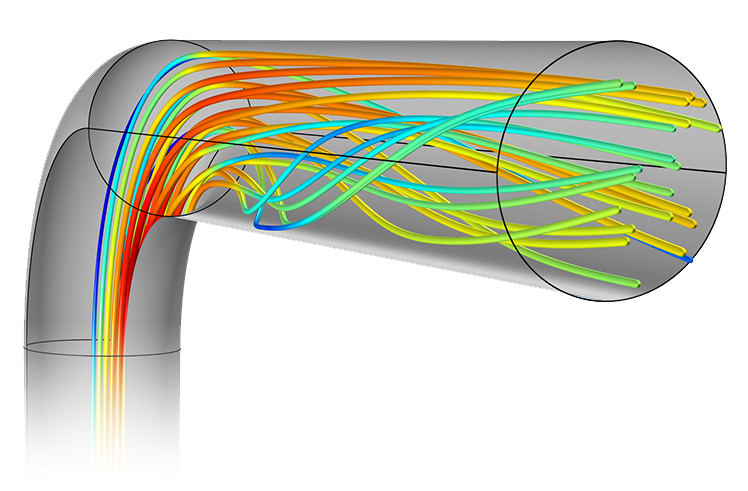
Fluid Dynamics of a Bent Pipe

Fluid Dynamics of a Bent Pipe#

Overview#

Computational Fluid Dynamics (CFD) simulations are an essential but computationally expensive and time-consuming process. Surrogate modeling using machine learning can greatly speed up predictions by approximating the simulation results. In this notebook, we compare two surrogate approaches:

A Fully Connected Feedforward Neural Network (FCFNN) baseline, treating each point independently.
A Graph Neural Network (GNN) surrogate, leveraging the spatial mesh as a graph.

We will train these surrogates on ground truth CFD data (outputs: turbulent kinetic energy, pressure, velocity) for a bent-pipe flow, and compare their performance using residual analysis, we will also compare their runtime to see which fits best for real-time monitoring for the pipe.

By the end of this project hopefully you will be able to see the utility of surrogate models in fluid dynamics.

Questions 1 & 2: Motivation for creating a surrogate model#

Question 01: CFD runtime#

Why do traditional CFD simulations take so long to run? visit Jose Alvarez and Mahmud Nobe’s notebook to learn more about the math that goes behind the scenes when using a CFD simulation (hint: the infamous Navier–Stokes equation)

(Answer here)

Data structure from the CFD simulation#

Training a surrogate model requires a large amount of data in the desired range, which is why we will use the data from this paper to train our model.

The system is a relatively simple bent pipe, structured as .txt files ranging from 0 to 200, with each file having a different velocity input towards the pipe. Each simulation file node data:

([nodenumber , x-coordinate, y-coordinate, z-coordinate, turb-kinetic-energy, pressure, temperature, velocity-magnitude]).

We drop the node index and filter out wall nodes (where velocity is zero) and we will ignore temperature. We then split into training and evaluation sets and compute normalization statistics.

!git clone https://github.com/lightiet/bended_pipe.git

Question 02: the 3 quantities #

Why is it important to monitor these 3 quantities in a system of interest? as a reminder they are

Turbulent Kinetic Energy (TKE)
pressure
velocity

(Answer here)

Data preparation#

!pip install -q torch-geometric
import time
from torch_geometric.data import Data
from torch_geometric.nn import GCNConv, knn_graph
from torch_geometric.utils import to_undirected
import torch.nn as nn
import torch.nn.functional as F
from torch.utils.data import Dataset, DataLoader
import torch
import os
import numpy as np
import matplotlib.pyplot as plt
from sklearn.neighbors import NearestNeighbors
torch.manual_seed(42)
np.random.seed(42)
rng = np.random.default_rng(seed=42)
device = torch.device("cuda" if torch.cuda.is_available() else "cpu")

Question 03: Data preprocessing#

Prepare the data for training.

think about the desired goal of this project, what should be the shape of the input and output vectors?

data_dir     = "bended_pipe/test_output_data"
file_pattern = "axial_output_{}.txt"
start_index  = 0
end_index    = 200  #
num_sims = end_index - start_index + 1
nodes_per_sim = 11340

# 1) Fill in the correct shape: (num_sims, nodes_per_sim, number_of_features)
#    Features here are: x, y, z, TKE, pressure, velocity
data_tensor = np.empty() # YOUR CODE HERE

for sim_idx, i in enumerate(range(start_index, end_index + 1)):
    fn  = os.path.join(data_dir, file_pattern.format(i))
    raw = np.loadtxt(fn, skiprows=1)           # shape (11340, 8)
    raw = raw[raw[:, 0].argsort()]              # sort by node number

    # 2) Select the correct columns for [x, y, z, TKE, pressure, velocity]:
    #    Remember: raw has columns [node#, x, y, z, TKE, pressure, temp, velocity]
    data_tensor[sim_idx] = raw[:,] # YOUR CODE HERE

# 3) Build a mask that drops any node where velocity (last feature) == 0:
mask = # YOUR CODE HERE
data_tensor = data_tensor[:, mask, :]
print("data_sorted!")

#segregate data to training and eval
perm      = rng.permutation(num_sims)
split_pt  = int(0.2 * num_sims)
eval_idx  = perm[:split_pt]
train_idx = perm[split_pt:]

train_tensor = data_tensor[train_idx]
eval_tensor  = data_tensor[eval_idx]

print("shape of the training tensor is" , train_tensor.shape)
print("shape of the evaluation tensor is" , eval_tensor.shape)

Reynolds Number (Re)#

The equation for Reynolds number is

\[ \Large Re = \frac{\rho U D}{\mu} \]

ρ is the density of the water
U is the flow velocity (usually taken at the inlet)
D is the diameter of the opening which is 0.025 m in our case
μ is the dynamic viscosity of the water.

This equation is especially important in fluid dynamics since it characterizes the regime of the system, when Re is high that means that the system is more turbulent and chaotic, and when Re is low the system is laminar and predictable.

def reynolds(U):
    return 87500 * U #in our case we only have one variable in the equation, U, the constants turn out to be 87500 after simplification

Question 04: Predictability and Re#

based on what you just read, what do you think the relationship between our surrogate model’s accuracy and Re will be?

(Answer here)

Visualizing understanding the data#

The following is a code snippet to visualize the data and help you gain intuition of what the data looks like

#mini helper function
def get_inlet_vel(sim_idx: int):
   return (data_tensor[sim_idx, 2, 5]) #3rd node's velocity is the inlet velocity

# 1) extract the velocity arrays for each simulation
velocities = data_tensor[:, :, 5]  # shape: (201, N_nodes)

# 2) compute per‐simulation statistics
max_vels = np.max(velocities, axis=1)  # highest velocity in each sim
min_vels = np.min(velocities, axis=1)  # lowest velocity in each sim

# 3) find the best (lowest max), worst (highest max), and the median‐case sim
best_idx   = np.argmin(max_vels)
worst_idx  = np.argmax(max_vels)

# for the median‐case, sort by max_vel and pick the middle simulation
sorted_by_max = np.argsort(max_vels)
median_idx    = sorted_by_max[len(sorted_by_max) // 2]

# collect indices for plotting
sim_indices = np.array([best_idx, median_idx, worst_idx])

var_names   = ['TKE', 'Pressure', 'Velocity']
case_labels = ['Re best case', 'Re 50% case', 'Re worst case']

vmins, vmaxs = [], []
for idx in range(len(var_names)):
    vals = data_tensor[sim_indices, :, 3 + idx]
    vmins.append(vals.min())
    vmaxs.append(vals.max())

for sim, label in zip(sim_indices, case_labels):
    # get inlet velocity and compute Reynolds number
    inlet_vel = get_inlet_vel(sim)
    Re_number = reynolds(inlet_vel)

    x = data_tensor[sim, :, 0]
    z = data_tensor[sim, :, 2]

    fig, axs = plt.subplots(1, len(var_names), figsize=(18, 5))
    for idx, name in enumerate(var_names):
        ax = axs[idx]
        values = data_tensor[sim, :, 3 + idx]
        sc = ax.scatter(
            x, z, c=values, s=10,
            vmin=vmins[idx], vmax=vmaxs[idx]
        )
        fig.colorbar(sc, ax=ax, label=name)
        ax.set_title(f"{name}")
        ax.set_xlabel("x")
        ax.set_ylabel("z")

    fig.suptitle(f"{label} (Re = {Re_number:.0f})", fontsize=16)
    plt.tight_layout(rect=[0, 0.03, 1, 0.95])
    plt.show()

Real-time monitoring of the pipe by ML#

Now that we’ve established that CFD models require significant computational resources, naturally they are not suitable for real-time prediction of a system’s state. This is where machine learning becomes valuable: by training models specifically on the geometry and outputs of our system, we can achieve accurate, real-time predictions.

Two approaches are presented below—try both and compare their performance.

Question 05: Fully Connected Feedforward Neural Network (FCFNN) approach#

let’s try the simplest method we have at our disposal, a FCFNN. Build an FCFNN that takes in the [x,y,z,U] and spits out [TKE, Pressure, Velocity]

To begin, we’ll load the data into a tensor and normalize it to prepare it for training.

coords_train = train_tensor[:,:,0:3].reshape(-1,3)
inlet_flat   = train_tensor[:,2,5].reshape(-1,1)  # velocity at node 2
Xcat = np.hstack([ np.repeat(coords_train, 1, axis=0),
                   np.repeat(inlet_flat, coords_train.shape[0]//inlet_flat.shape[0], axis=0) ])
Y_flat = train_tensor[:,:,3:6].reshape(-1,3)

mu_in,  s_in  = Xcat.mean(axis=0), Xcat.std(axis=0)  + 1e-8
mu_out, s_out = Y_flat.mean(axis=0), Y_flat.std(axis=0) + 1e-8

norm_stats = (
    torch.tensor(mu_in,  dtype=torch.float32),
    torch.tensor(s_in,   dtype=torch.float32),
    torch.tensor(mu_out, dtype=torch.float32),
    torch.tensor(s_out,  dtype=torch.float32)
)

Now we have

mu_in, s_in

which are the per‑feature mean and standard deviation of inputs [x, y, z, U]

mu_out, s_out

which are the per‑feature mean and standard deviation of targets [TKE, Pressure, Velocity].

class FCFNN(nn.Module):
    #YOUR CODE HERE
model = 
torch.save(model.state_dict(), 'fcfnn_checkpoint.pth')

Question 06: Graph neural networks#

Treat each mesh point in the CFD simulation as a node whose behavior is influenced by its neighbors, and capture these local interactions with a graph neural network. Construct a GNN that first builds a K‑nearest‑neighbor graph based on the 3D coordinates, then processes the normalized input features[x,y,z,U] through an encoder, several graph‑convolution layers, and a decoder to predict the three target fields [TKE, Pressure, Velocity] just like the FCFNN.

Be sure to standardize both inputs and outputs before training.

SEED = 42
hidden_dim     = 128
num_layers     = 3
learning_rate  = 1e-3
epochs          = 15
batch_size      = 1
k_neighbors     = 6      # for KNN graph

def build_knn_graph(coords, k):
    """
    Given coords of shape (N,3), build a 2xE edge_index tensor
    connecting each node to its k nearest neighbors (excluding itself).
    Returns: torch.LongTensor edge_index
    """

class FlowDataset(Dataset):
    def __init__(self, data_tensor, mask=None, norm_stats=None):
        self.data = data_tensor
        self.mask = mask
        self.mu_in, self.s_in, self.mu_out, self.s_out = norm_stats
        # coords identical for every sim
        self.coords = torch.tensor(data_tensor[0,:,:3][mask], dtype=torch.float32)
        self.edge_index = build_knn_graph(self.coords.numpy(), k_neighbors)
    def __len__(self):
        return self.data.shape[0]

    def __getitem__(self, idx):
        arr = self.data[idx]
        # 2) Extract xyz positions and inlet velocity and normalize inputs (x) and outputs (y)

        # YOUR CODE HERE

        return x, y, self.edge_index

def collate_graph(batch):
    return batch[0]

class GraphConvLayer(nn.Module):
    def __init__(self, dim):
        super().__init__()
        # Initialize linear layers for self‑ and neighbor contributions
        # YOUR CODE HERE

    def forward(self, h, edge_index):
        #implement message passing
        # YOUR CODE HERE


class FlowGNN(nn.Module):
    def __init__(self, in_dim=4, hidden_dim=128, out_dim=3, n_layers=3):
        super().__init__()
        # 1) Define an encoder to map input features to hidden_dim
        # 2) Create a sequence of GraphConvLayer modules
        # 3) Define a decoder to map back to output dimension

        # YOUR CODE HERE

    def forward(self, x, edge_index):
        # implement GNN forward
        # YOUR CODE HERE

Now create a training loop

train_set = FlowDataset(train_tensor, mask, norm_stats)
train_loader = DataLoader(train_set, batch_size=batch_size, shuffle=True)
model = FlowGNN().to(device)
optimizer = torch.optim.Adam(model.parameters(), lr=learning_rate)
criterion = nn.MSELoss()
for epoch in range(1, epochs+1):
    #YOUR CODE HERE

torch.save(model.state_dict(), 'gnn_checkpoint.pth')

Question 07: Visualizing the output of the models#

Implement a function predict_fields(U) that, given an inlet velocity U and model GNN or FCFNN, computes and returns the model’s predicted field values across the entire pipe.

def predict_fields(U: float, model_type: str) -> np.ndarray:
    """
    Given inlet velocity U, returns an (N, 6) array:
    [x, y, z, TKE_pred, pressure_pred, velocity_pred]
    """
    if model_type.upper() == "GNN":
        ckpt = torch.load("flow_gnn_checkpoint.pt", map_location=device)
        model = FlowGNN(in_dim=4, hidden_dim=hidden_dim, out_dim=3, n_layers=num_layers)
    elif model_type.upper() == "FCFNN":
        ckpt = torch.load("fcfnn_checkpoint.pt", map_location=device)
        model = FCFNN(input_dim=4, hidden_dims=(hidden_dim,)*num_layers, output_dim=3) #you might want to change these values to match your model
    else:
        raise ValueError(f"Unsupported model_type: {model_type}")

    model.load_state_dict(ckpt['model_state_dict'])
    model.to(device).eval()
    mu_in, s_in, mu_out, s_out = ckpt['norm_stats']

    coords_np  = data_tensor[0, :, :3].astype(np.float32)
    edge_index = build_knn_graph(coords_np, k_neighbors).to(device)

    N = coords_np.shape[0]
    U_col = np.full((N, 1), U, dtype=np.float32)
    X_raw = np.hstack([coords_np, U_col])
    X_norm = (X_raw - mu_in.cpu().numpy()) / s_in.cpu().numpy()

    x_t = torch.from_numpy(X_norm).float().to(device)

    with torch.no_grad():
        if model_type.upper() == "GNN":
            out_norm = model(Data(x=x_t, edge_index=edge_index))
        else:
            out_norm = model(x_t)

    # De-normalize outputs
    Y_pred = (out_norm.cpu().numpy() * s_out.cpu().numpy()) + mu_out.cpu().numpy()

    # Return stacked coords + predictions
    return np.hstack([coords_np, Y_pred])

Now we are ready! with the simple call of a function and an input of inlet velocity, we can get the profile for the whole pipe.

Now let’s test the run time and plot an example.

Question 08: Evaluation of the models #

# Time GNN prediction
start = time.perf_counter()
gnn_output = #YOUR CODE HERE
end = time.perf_counter()
print(f"GNN predict_fields took {end - start:.6f} seconds")

# Time FCFNN prediction
start = time.perf_counter()
fcfnn_output = #YOUR CODE HERE
end = time.perf_counter()
print(f"FCFNN predict_fields took {end - start:.6f} seconds")

# plot outputs
var_names = ['TKE', 'Pressure', 'Velocity']
model_outputs = [gnn_output, fcfnn_output]
model_labels = ['GNN', 'FCFNN']

for model_out, model_label in zip(model_outputs, model_labels):
    x = model_out[:, 0]
    z = model_out[:, 2]

    fig, axs = plt.subplots(1, len(var_names), figsize=(18, 5))
    for idx, name in enumerate(var_names):
        ax = axs[idx]
        values = model_out[:, 3 + idx]
        sc = ax.scatter(x, z, c=values, s=10)
        fig.colorbar(sc, ax=ax, label=name)
        ax.set_title(f"{model_label} - {name}")
        ax.set_xlabel("x")
        ax.set_ylabel("z")

    fig.suptitle(f"{model_label} Single Simulation Visualization", fontsize=16)
    plt.tight_layout(rect=[0, 0.03, 1, 0.95])
    plt.show()

As you can see this is quite powerful, we no longer need to compute the profile of the pipe using CFD anymore, we can just call the predict_fields function and we will get what we need in an instant!

now before we use this model to monitor our pipe, we should check for validity, the code below shows the loss in each of the 4 outputs.

sim   = 0
U_val = 0.69
ε     = 1e-8 #to avoid accidental division by 0
coords_np = data_tensor[0, :, :3].astype(np.float32)

# Ground truth
actual    = data_tensor[sim, :, 3:6]

# Predictions
gnn_pred    = predict_fields(U_val, "GNN")[:, 3:6]
fcfnn_pred  = predict_fields(U_val, "FCFNN")[:, 3:6]

# Compute relative errors: |pred - true| / (|true| + ε)
gnn_rel_err   = np.abs(gnn_pred   - actual) / (np.abs(actual) + ε)
fcfnn_rel_err = np.abs(fcfnn_pred - actual) / (np.abs(actual) + ε)

for rel_err, label in [(gnn_rel_err, "GNN"), (fcfnn_rel_err, "FCFNN")]:
    x = coords_np[:, 0]
    z = coords_np[:, 2]

    fig, axs = plt.subplots(1, len(var_names), figsize=(18, 5))
    for idx, name in enumerate(var_names):
        ax = axs[idx]
        sc = ax.scatter(
            x, z,
            c=rel_err[:, idx],
            s=10,
            cmap='viridis'
        )
        fig.colorbar(sc, ax=ax, label=f"{name} Relative Error")
        ax.set_title(f"{label} – {name} Rel. Error")
        ax.set_xlabel("x")
        ax.set_ylabel("z")

    fig.suptitle(f"{label} Relative Error Field", fontsize=16)
    plt.tight_layout(rect=[0, 0.03, 1, 0.95])
    plt.show()

From the results above, which NN works best for this use case?

(Answer here)

Question 09: Relationship between Re and loss #

Write a breif scrip that plots Re vs model loss for both models over the evaluation simulations.

#YOUR CODE HERE

Was your initial guess about the relationship between Re and the model’s accuracy correct?

(Answer here)

Question 10: Possible improvements (optional) #

What enhancements or modifications would you suggest for these surrogate models?

Is there another technique that you think will work better? feel free to test it down below.

Acknowledgements#

Initial version: Abdulaziz Alshohail with some guidance from Mark Neubauer

Fluid Dynamics of a Bent Pipe

Contents

Fluid Dynamics of a Bent Pipe#

Overview#

Questions 1 & 2: Motivation for creating a surrogate model#

Question 01: CFD runtime#

Data structure from the CFD simulation#

Question 02: the 3 quantities #

Data preparation#

Question 03: Data preprocessing#

Reynolds Number (Re)#

Question 04: Predictability and Re#

Visualizing understanding the data#

Real-time monitoring of the pipe by ML#

Question 05: Fully Connected Feedforward Neural Network (FCFNN) approach#

Question 06: Graph neural networks#

Question 07: Visualizing the output of the models#

Question 08: Evaluation of the models #

Question 09: Relationship between Re and loss #

Question 10: Possible improvements (optional) #

Acknowledgements#